AI Fairness (Approaches & Mathematical Definitions)

12 min readJan 3, 2022

What is fair? Can we define fairness in mathematical equations? In this article, we will approach these definitions systematically and establish a framework for the problems if possible. We will also look into more advance topics including counterfactual fairness.

Notation

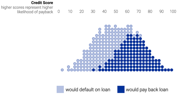
To discuss the topic, let’s start with an example that uses predicted credit scores to approve car loans. We will introduce the notations we need in this article. On the top of the diagram below is the credit score R (0 to 100) for each loan. A few years later, we would discover whether loans are paid back or not: the dark blue dots indicate they are paid back and the light blue dot loans would default.

x is the information of an applicant. A indicates the group membership (say the gender). Y is the outcome/ground truth on whether a loan will be paid back.

The model predicts a credit score R. If it is higher than a threshold t, the bank will make a decision D=1. The loan is approved.

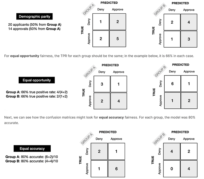
Here is an example of the confusion matrix (Actual Y v.s. Predicted: D):

Bayes optimal score is:

In some of the optimized models, we want to predict this score faithfully.

Statistical Fairness Criteria

Here is a sample list of fairness criteria. We will look into some of them here.

Equalizing acceptance rate

Both group “a” and group “b” will have the same acceptance rate. So if group a has an acceptance rate (positive rate) of 63%, so does group b.

“Equalizing acceptance rate” is also called statistical parity or demographic parity.

Sometimes, we can give it some slack. The four-fifths rule states that the chance of acceptance for the disadvantaged group should be at least within 80% of the other group (ε=0.2).

Here is in another form.

This can be done by pre-processing which learns a latent feature Z that is independent of A ( Z ⊥ A.).

Here is an approach in this paper that maximizes the mutual information of the input features given Z while minimizing the mutual information of A given Z. i.e. knowing Z should have very limited information on A. Here are other papers on similar approaches (1, 2), But as a warning, what it achieves is Z ⊥ A. That does not imply it is a fair representation of the input.

“Equalizing acceptance rate” fits into a more general criterion called independence that

If the independence criterion is fulfilled, “equalizing acceptance rate” will be true also and the acceptance probabilities will be the same. If we have R to be independent of A, the model will achieve the same acceptance rates also.

There are other ways to achieve independence, like post-processing and the training time constraint.

Indedepency ignores the possible correlation between A and Y. For example, there is an imbalance between male and female sushi chefs. So even if we retarget the ads to both genders fairly, this criterion may still be unfulfilled. This rules the most optimal predictor where D = Y. The solution will be suboptimal compared with the unconstrained model.

Will the criterion rule out unfairness? Consider a lazy manager. He/she works hard in group “a” to find all the true positives. But to meet the same acceptance quota, he/she simply makes random decisions in group b such that the group will have the same proportion of approved loans. We need safeguards for the ML model so the objective is not achieved through laziness.

By intention or not, both groups below have the same positive rates. But no justice is done to group b. Group a and b are not treated equally. Trading true positives with false positives does not mean fairness.

So even with the same acceptance rates, there is no guarantee that justice is done. In some situations, to enforce this constraint, it may hurt group “a” instead.

But it does not imply it is useless. We will come back to this later.

Equalizing error rate

In Equalizing error rate, we want the error rates to be the same for both groups. Unlike Equalizing acceptance rate, we cannot trade true and false positives anymore.

If creditworthy persons in a group have a higher rate of being misjudged than other groups, they may feel unfair. In equalizing the error rate, the misclassification rates among all groups are the same. Such unfairness will not occur.

We can also evaluate the score function by plotting its ROC curve. This curve plots the TPR against FPR for all possible thresholds. It summarizes the performance of the score function. The 45° line is when the model is just random guessing. It is equally likely to make right and wrong decisions.

The following is the ROC curve for group “a” (green) and “b” (blue). The shaded area, where both curves intersect, are all the tradeoffs that are achievable under all groups (that are the tradeoffs that can be achieved by some thresholding at each group). So if we have the cost for the false positives and false negatives, we can search over this region and pick the tradeoff that we like the best for the cost we have. Here is the paper on using post-processing with group-sensitive thresholding. The basic idea in post-processing is to find a proper threshold using the score R (R is not group sensitive) for different groups.

Alternatively, we can add a constraint to the objective function in the training time. The solution below is highly intractable. This paper will have more information on how to solve it.

Equalizing error rate fits into a more general criterion called separation.

Again, we can have R to be independent of A given Y. It will achieve equalizing error rate also. Unlike independence, separation allows A and Y to be correlated. As it allows D = Y, the model can be as optimal as the unconstrained model. It also penalizes laziness as it wants to achieve uniform error rates in all groups.

Error rate parity is a post-hoc criterion. We can collect past loan data to see if they have been paid back or they are default. And we can use that data to see how a classifier is doing. Obviously, at the loan decision time, this information is unknown until many years later.

Equalized odd/Equal opportunity

Equalized odd is related to separation also.

In equalized odd, a person should have the same odd of a decision D regardless of which group they are in. Each group has the same true positive rate TPR and the same false negative rate. So if you are qualified (or not qualified), applicants from each group should have the same odd to be hired.

This definition cannot close the hiring gap between a and b if the disadvantaged group has less qualified applicants. Some people may argue that if given a chance, they will do as well as others.

Calibration

A score r is calibrated if:

score 0.7 means 0.7 chance of positive outcomes on average over people who receive score 0.7. Score value r corresponds to positive outcome rate r. Note: this does not indicate an individual will have a chance r for a positive outcome.

A score r is calibrated by group if:

Here is one of the methods in achieving calibration through the Platt scaling. Here, we fit the sigmoid function below against the target Y.

Calibration by group fits into a more general criterion called sufficiency.

So R is sufficient enough to predict Y. The knowledge of A is not needed.

Calibration is an “a priori” guarantee. If a decision-maker sees a score value r, he/she will know the frequency of positive outcomes.

In the US, it is illegal to discriminate against a qualified individual with a disability in employment. Such disability is considered morally irrelevant. But group calibration will not resolve such moral irrelevant

Predictive parity

Predictive parity is also related to sufficiency. In predictive parity, both groups will have the same precision. i.e. for all the positives they predicted, they have the same proportions that the predictions are correct (true positive). Mathematically, it is defined as:

Independency, Separation, Sufficiency

There are other fairness criteria, but they are related to independency, separation, or sufficiency.

Here comes the bad news. Can we have an application that satisfies all criteria ( independency, separation, and sufficiency) simultaneously? The answer is no. Any two of these criteria are mutually exclusive in general. Assuming both groups has unequal base rates: P(Y=1 | A = a) ≠ P(Y=1 | A = b) and the model makes imperfect decisions (the error rates for D is greater than 0). Then, calibration by group implies that error rate parity fails.

Confusion matrix

Here is another perspective of viewing these definitions from the perspective of confusion matrix using true/false positive, true/false negative, true positive rate, and true negative rate.

Individual Fairness

The fairness criteria discussed so far belong to group fairness. In group fairness, we ask the question of whether it is fair to different groups. Instead of putting individuals into groups, individual fairness asks whether similar individuals get similar outcomes (paper).

So given two sample points, d is the metric measuring the dissimilarity between two individuals on a specific task. For example, what is the dissimilarity of two individuals in applying for a job: what is the difference in education, experience, etc …

x will map to a probability distribution M(x) for the outcome. For example, M(x) is the probability distribution of getting hired for x.

In individual fairness, we want the difference in outcome distribution D(M(x), M(x’)) to be smaller or equal to d(x, x’).

This paper adds a dissimilarity in the “construct space” to improve the concept.

In addition to characterizing the spaces of inputs (the “observed” space) and outputs (the “decision” space), we introduce the notion of a construct space: a space that captures unobservable, but meaningful variables for the prediction.

Counterfactual Fairness

Technological advances, like contextual fairness, may help us to do better. Here is a quote from a contextual fairness paper.

It allows us to propose algorithms that, rather than simply ignoring protected attributes, are able to take into account the different social biases that may arise towards individuals based on ethically sensitive attributes and compensate for these biases effectively.

Many scholars (1, 2) have argued that the most optimal and fair solutions would require all factors considered. Otherwise, it constrains how ML can advance equal outcomes.

In counterfactual fairness, we ask a simple question: if we change the gender of an applicant from male to female, will the applicant be more likely or less likely to be accepted. Let’s explain it in an easy-to-understand way. Here is a case study in the paper.

The Law School Admission Council conducted a survey across 163 law schools in the United States. It contains information on 21,790 law students such as their entrance exam scores (LSAT), their grade-point average (GPA) collected prior to law school, and their first year average grade (FYA). Given this data, a school may wish to predict if an applicant will have a high FYA. The school would also like to make sure these predictions are not biased by an individual’s race and sex. However, the LSAT, GPA, and FYA scores, may be biased due to social factors.

So race and sex are the sensitive characters A that cause systematic bias. Some races may do better economically. They can afford special test preparation classes to improve their LSAT score. When we predict FYA, we want to separate factors related to race and factors not related to race.

The observable variable x includes LSAT and GPA. FYA is the score Y we want to predict. Here is one possible casual model M on the problem. As shown, race can impact GPA, LSAT, and FYA.

Source (one possibility for the Casual Model M)

Now, we introduce Know (K). It impacts GPA, LSAT, and FYA. This is the fair variable U that we want to model and learn. It is called fair because it does not depend on race or sex. We don’t know what K is. It is the unobservable latent variable. Like other ML problems, we want to learn from the data. Since it does not depend on sensitive characters, K captures the non-racial or gender-neutral information that influences FYA. To make fair decisions, we should make decisions based on K only.

Mathematically, Counterfactual Fairness is:

If we switch the race from male to female, it should give the same probability distribution on Y (FYA score).

There are different ways to build the casual model M based on different assumptions and simplifications. Just for demonstration, we will discuss the level 2 model in the paper. (refer to the paper for details.)

In this model, we will use the distributions below in modeling the dependency demonstrated by the edge. With data samples, we can learn the model parameters below (b, w).

Source

So given M and the dataset D, we can sample the value of fair variable U (Know) for samples in D. Then, we can train a model Y parameterized by θ to predict FYA from U only. There are more details in the algorithm below but the fine details are not important for our discussion here.

To make a prediction, we compute U for an individual using M and then predict FYA from θ. Here is a video that discusses counterfactual fairness in more detail if you need it.

Fairness is a huge topic. We are just showing a small segment of the topic. Here is a course and a 2-hour lecture in fairness that may interest you.