AlphaGo Zero — a game changer. (How it works?)
Even AlphaGo is impressive, it requires bootstrapping the training with human games and knowledge. This is changed when DeepMind released AlphaGo Zero in late 2017. While it receives less media attention, the breakthrough may be more significant. It is self-trained without the human domain knowledge and no pre-training with human games. This brings us one step closer to what Alan Turing may vision:
Instead of trying to produce a programme to simulate the adult mind, why not rather try to produce one which simulates the child’s?
We may expect AlphaGo Zero is more complicated and harder to train. Ironically, AlphaGo Zero has only one deep network and takes only 3 days of training to beat AlphaGo which takes 6 weeks of training.
AlphaGo Zero Deep network
In reinforcement learning (RL), we use a policy p to control what action should we take, and a value function v to measure how good to be in a particular state.
In Go, our policy controls the moves (actions) to win a game. To model uncertainty, the policy is a probability distribution p(s, a): the chance of taking a move a from the board position s. The value function is the likeliness that we will win from a specific board position. As an example below,
- the probability of taken move a3 is 0.6, and
- at the board position s’3, the value function is 0.9. i.e. a 0.9 chance of winning the game.

In AlphaGo Zero, we use a single deep network f, composed of convolutional layers, to estimate both p and v.
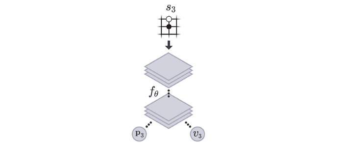
It takes the board position (s) as input and outputs p and v accordingly.

In the original AlphaGo, it uses two separate deep networks, and we train them with human-played games using supervised learning. In AlphaGo Zero, we train a single network f using self-play games. However, learning the policy and the value function is not good enough (or accurate enough) to beat the Go masters. We need the Monte Carlo Tree Search (MCTS). We will look into MCTS first before coming back on how the deep network f is trained.
Monte Carlo Tree Search (MCTS)
In MCTS, we use a search tree to record all sequence of moves that we search (play). A node represents a board position and an edge represents a move. Starting with a board position (s3 below), we search possible moves and evaluate the policy and the value function using the deep network f.

We estimate position s’3 has a 0.9 chance of winning (v=0.9). We expand the search tree by making a move. This adds a new board position and its corresponding moves to the search tree. We use f to estimate the value function and the policy for the added node and edges.

(To reduce confusion in our discussion, the value function is relative to us rather than the current player or the opponent.)
Let’s introduce another term called action-value function Q. It measures the value of making a move. In (a) below, we take the move in red (a3) and end up with a 0.9 chance of winning. So Q is 0.9. In (b), we make one more move and end up with a 0.6 chance of winning. Now, we have taken the move a3 twice (visit count N=2). The Q value is simply the average of previous results, .i.e. W=(0.9+0.6), Q = W/2=0.75. In (c), we explore another path. Now, a3 is picked 3 times and the Q value is (0.9+0.6+0.3)/3 = 0.6.
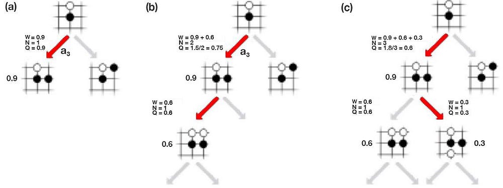
The Q value serves a similar purpose as the policy p estimated by the deep network f. However, as we explore more, our search tree grows bigger. If we play enough, the noise in p cancel each other. So Q is getting more accurate as we make more moves.
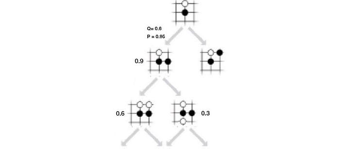
However, the search space for Go is huge, we need to prioritize our search better. There are two factors we need to consider: exploitation and exploration.
- exploitation: perform more searches that look promising (i.e. high Q value).
- exploration: perform searches that are not frequently explored (i.e. low visit count N).

Mathematically, we select the move a according to:

where u is

In this equation, Q controls the exploitation and u (inverse to its visit count) controls the exploration . Starting from the root, we use this policy (tree policy) to select the path that we want to search further.
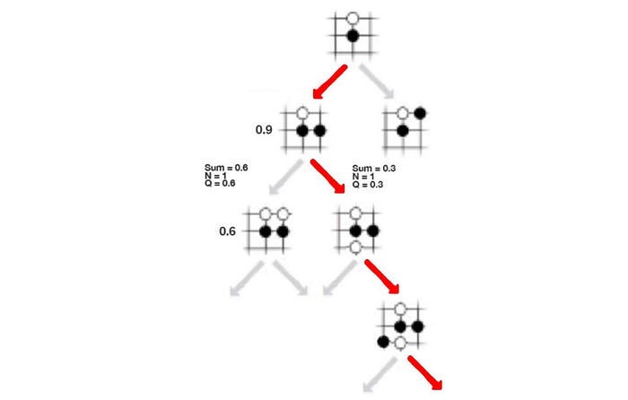
In the beginning, MCTS will focus more on exploration but as the iterations increase, most searches are exploitation and Q is getting more accurate.
AlphaGo Zero iterates the steps about 1,600 times to expand the tree. We use the search tree to create a policy π to pick our next move for the board position s3.

Surprisingly, we do not use Q to compute the policy π. Instead, π is derived from the visit count N.


After the initial iterations, moves with higher Q value will be visited more frequently. We use the visit count to calculate the policy because it is less prone to outliners. τ is a temperature controlling the level of exploration. When τ is 1, we select moves based on the visit count. When τ → 0, only the move with the highest count will be picked. So τ =1 allows exploration while τ → 0 does not.
With a board position s, MCTS calculates a more accurate policy π to decide the next move.

MCTS improves our policy evaluation (improves Q), and we use the new evaluation to improve the policy (policy improvement). Then we re-apply the policy to evaluate the policy again. These repeated iterations of policy evaluation and policy improvement are called policy iteration in RL. After self-playing many games, both policy evaluation and policy improvement will be optimized to a point that it can beat the masters. (A recap of the MCTS can be found here.)
Difference between AlphaGo and AlphaGo Zero search algorithm
As shown below, AlphaGo does not use the Monte Carlo Rollout (in yellow).
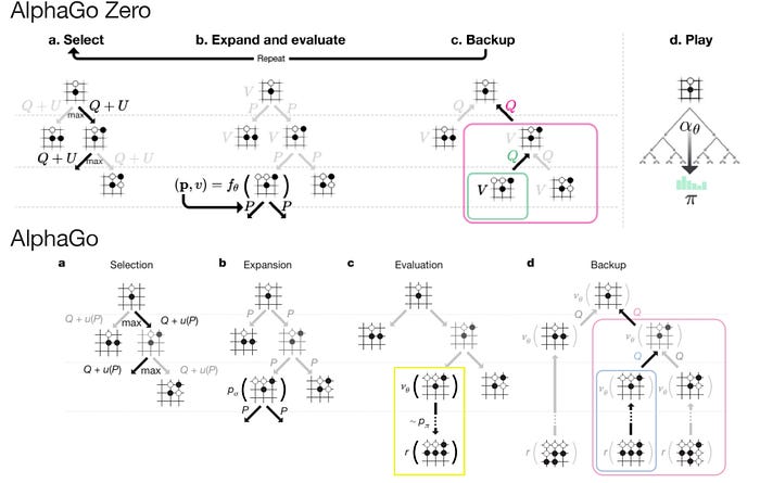
AlphaGo Zero uses the self-trained network θ to calculate the value function v while Alpha Go uses the SL policy network σ learned from real games. Even the equation in computing Q looks different, the real difference is AlphaGo has an extra term z (the game result) that is found by the Monte Carlo rollout which AlphaGo Zero skips.

Self training using Monte Carlo Tree Search
After looking into MCTS, we come back on how f is trained. So we start with an empty board position s1. We use the MCTS to formulate a policy π1. Then we sample a move a1 from π1. After taking the move a1, the board is in s2. We repeat the process again until the game is finished at which we determine who win z (z=1 if we win, 0 otherwise.).

This whole self-play game creates a sequence of input board position, policy and game result z.

This is the dataset we used to train the deep network f using supervised training. AlphaGo Zero plays games with itself to build up a training dataset. Then it randomly selects samples from the dataset to train f.
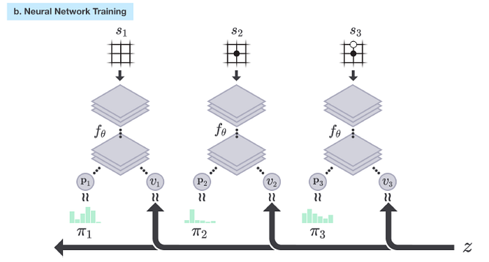
Our loss function used in the training contains:
- a mean square error between our value function estimation v and the true label z.
- A cross entropy for the estimated policy p and the policy π, and

- a L2 regularization cost with c = 0.0001.

Self-Play Training Pipeline
However, not all self-play games are used for the deep network f training. Only games played by the best models are used. This self-play training pipeline contains 3 major components that run concurrently.
- Optimization: Using samples in the training dataset to optimize f and checkpoint models every 1,000 training iterations.
- Evaluator: If the MCTS using the new checkpoint models beats the current best model, we use it as the current best model instead.
- Self-play: Play 25,000 games with the current best model and add them to the training dataset. Only the last 500,000 self-play games are kept for training.
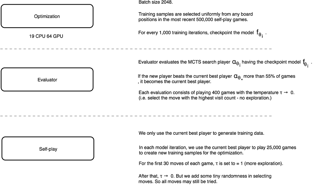
AlphaGo Zero was trained for 40 days with 29 million self-play games. The parameters for f are updated from 3.1 million of mini-batches each containing 2,048 board positions.
Recap
The deep network f is trained concurrently when AlphaGo is playing games with itself. Using the policy and the value estimation from the network f, MCTS builds a search tree to formulate a more precise policy for the next move. In parallel, AlphaGo Zero let MTCS plays against each other using different versions of the deep network f. Then it picks the best one so far to create the training samples needed to train f. Once the training is done, we can use the MCTS with the most optimal network f to plan for the next move in a real game.
Deep network architecture
The deep network f composes of a 3×3 convolutional layer outputting 256 channels followed by 39 residual blocks. A residual block composes of 3×3 convolutional layers and skip connections.
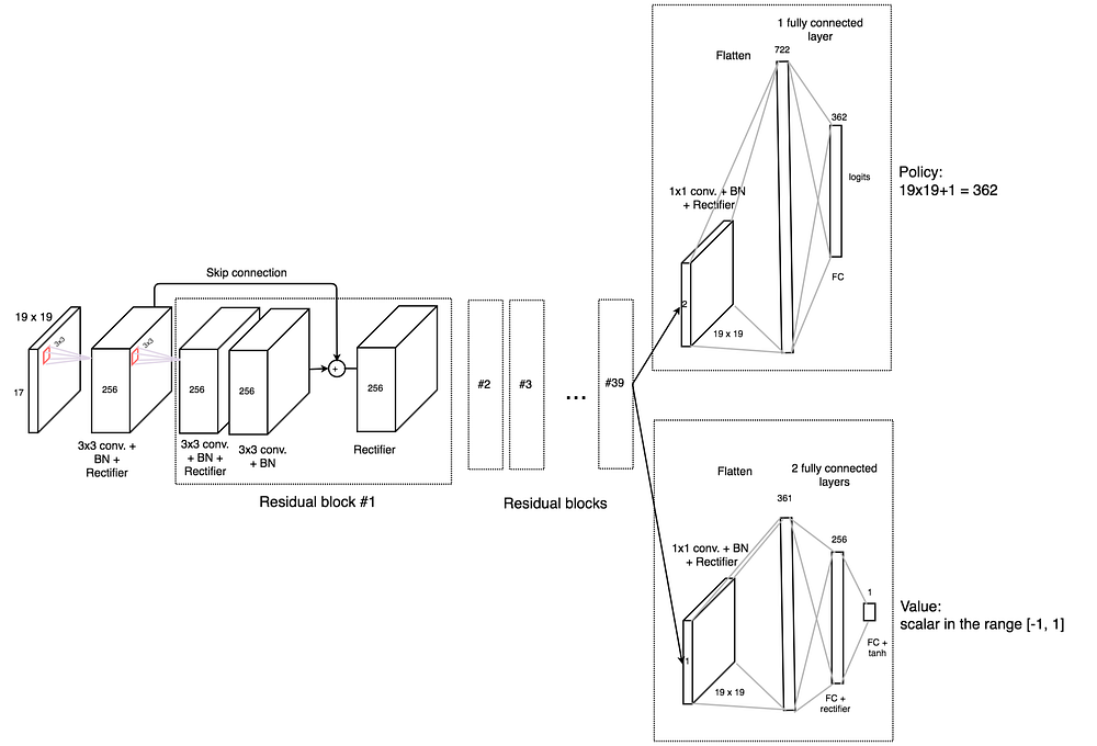
The output is feed into a policy head and a value function head.
- The policy head composes of a 1×1 convolutional layer output 2 channels. The layer is flatten to a vector of 722 elements followed by a FC layers outputting 362 logits (move to one of the 19×19 possible locations, or pass).
- The value head composes of a 1×1 convolutional layer output a single channel. The layer is flatten to a vector of 361 elements followed by a FC layer outputting 256 elements, then another FC layer to a scalar value followed by tanh (output values between -1, 1).
The network takes an input of 19×19×17 features (17 features for each grid location for the 19×19 Go board). The input features contain the current and the last 7 board positions (a total of 8 positions). For each grid location, it has 2 binary values: the presence of the white and the black stone respectively. Therefore we have a total of 8×2=16 features. The last feature is the color of the stone to play now.
Reference
Symmetry

Since a Go board is symmetrical, we can randomly rotate or mirror a board with the function d in our training. This acts as a kind of data augmentation.
End of game
A game is finished when
- both players pass, or
- the search value drops below a resignation threshold, or
- the game exceeds a maximum time step.
The game is scored to determine who win.
Further reading
How the original AlphaGo works.
Credits
Diagrams in particular containing

are modified from the original DeepMind’s “Mastering the Game of Go without Human Knowledge” paper.
