Bias in Clinical Research, Data Science, Machine Learning & Deep Learning

In 2016, Democrat’s models projected a 5-point win over Michigan through Presidential Election Day. And models for other must-win states made similar predictions.

The rest were history. Clinton lost the US presidential election.
Data is a critical part of our life. What we read or what we watch depends on them. Many recommender systems are so optimized for engagement that they sow division, misinformation, or worse extremism. It becomes so abusive that we should not turn a blind eye to AI biases anymore. But, bias in data is nothing new. This is heavily studied in clinical research, data science, and business school. And there are plenty of articles on the ethical impacts on AI. So, in our discussion, we will focus on the technical perspective only. Some of these biases are so obvious that they should never happen. But it does — even plenty of them in professional studies.
In the first part of the article, we look into the common biases in clinical research and data science. Since the medical field is a major candidate for AI applications, we will spend some time on its corresponding bias in data collection. For the rest of this series, we will study the impact of bias on AI applications, fairness, and AI governance.
First, let’s look at an example of data analysis. Paul is a renowned high school football coach and moved to Seattle a few years ago. Since Seattle rains a lot, he decided to have his team focused on the running game. He collects the statistics for the last few years and checks whether his strategy is working. Here, we have two variables A and B here. A represents rain and ~A represents not rain. B represents the team wins and ~B represents otherwise. The table contains counts accounting for different combinations of A and B. So from this table, what conclusion you may draw.

One common conclusion is Paul's strategy is winning. He wins 32 games when raining. This conclusion draws from the fact that count(A, B) is far much higher than other scenarios. But this conclusion is wrong.

On the contrary, Paul’s team has a marginally higher chance of winning when it is not raining. We can explain this in plain English. The high count is simply because Seattle rains a lot, and Paul is a good coach that wins a lot too. The frequency of A and B fool many people to the wrong conclusion. Things that happen together often do not necessarily mean they are correlated. In this example, it's just Paul wins often and Seattle rains often. So don’t take too much advice from Seattleite about what happens when raining.
There are many probability brain teasers that use an unusual high P(A) and P(B) to throw people off. So, don’t jump to conclusions too fast. But it also demonstrates a common real-life misconception. We need to realize that the most happen combination does not necessarily mean they have a positive correlation.
Note: bias is a huge topic. Depending on the field of studies, they may be described with different terms. Some biases can be classified using different categories since it is not easy to draw where the boundary is. (Or they can belong to multiple groups.) This article is just a starting point and we encourage you to study it further if interested.
Now, we introduce the first kind of bias — who are we collecting data from.
Selection Bias
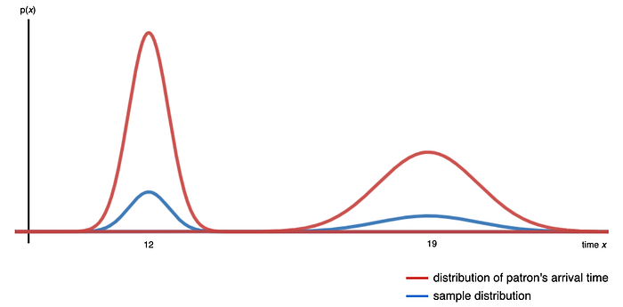
We sample from a population of interest to draw conclusions. The diagram below shows the distribution of the patron’s arrival time at a restaurant. If we want to draw a conclusion, like the average tips from a patron, we sample patrons randomly. If the distribution of the sampled patrons (in blue) is not proportional to the distribution of the restaurant patrons (in red), our conclusion will be inaccurate, this is the selection bias. The collected samples do not represent the population of interest.
Sampling Bias happens when not every case in the population will have an equal likelihood to be chosen. How to sample data randomly remains elusive in many studies, even worse in deep learning. Here is a Science article on using neural network NN in identifying pneumonia from X-rays in 2017.
But Eric Oermann, a neurosurgeon at Mount Sinai Hospital in New York City, has explored one downside of the algorithms: The signals they recognize can have less to do with disease than with other patient characteristics, the brand of MRI machine, or even how a scanner is angled. With colleagues, Oermann developed a mathematical model for detecting patterns consistent with pneumonia and trained it with x-rays from patients at Mount Sinai. The hospital has a busy intensive care unit with many elderly people, who are often admitted with pneumonia; 34% of the Mount Sinai x-rays came from infected patients.
…
At Mount Sinai, many of the infected patients were too sick to get out of bed, and so doctors used a portable chest x-ray machine. Portable x-ray images look very different from those created when a patient is standing up. Because of what it learned from Mount Sinai’s x-rays, the algorithm began to associate a portable x-ray with illness. It also anticipated a high rate of pneumonia.
In a nutshell, the algorithm associates the portable x-ray device with pneumonia — such association improves the accuracy of the model! In hindsight, we should be aware of all these variables, including the type of machine, manufacturer, etc … But this is usually more complex than we realize. Often, we realize the issues after the fact. For now, it is too difficult in interpreting what a NN model learns and we declare victory too early.
Let’s look into details on different types of selection bias.
Time is another variable that we often ignore. Clearly, we cannot study the S&P 500 return by collecting samples from one year of data only. That explains why there are young traders who gamble and lose billion dollars for their investment firms. They know finance well but these traders are vulnerable to market downturns because they never experience a recession. In designing an experiment, its duration and how responsive the measures are, with respect to time, are important. For example, in an e-commerce experiment, the add-to-cart ratio is more responsive than the gross merchandise value (GMV). In many software platforms, releases are made even daily. We may depend on proxy measurements in our experiments (an indirect measure of the target outcome which is itself strongly correlated to that outcome). But yet, it may introduce bias.
Attrition bias may happen when some participants do not complete the study and therefore, their data is not added to the final result. For example, when patients find an experimental drug is not effective, they may drop off from the study prematurely. With these cases dropped, the final result may appear to be more impressive than it should be. Other reasons for the dropout may include adverse effects of the drug or clinical improvements.
Survivorship bias happens when we only examine subjects that still survive when the test is done. Nictoine stimulates brain. So, does smoking reduce dementia? Here is the quote from a research paper:
The relative rate for smokers versus nonsmokers ranged from 0.27 to 2.72 for Alzheimer disease (12 studies) and from 0.38 to 1.42 for dementia (6 studies). The minimum age at entry (range: 55–75 years) explained much of the between-study heterogeneity in relative rates. We conjecture that selection bias due to censoring by death may be the main explanation for the reversal of the relative rate with increasing age.
In short, some smokers die before dementia symptoms appear. This creates a bias.
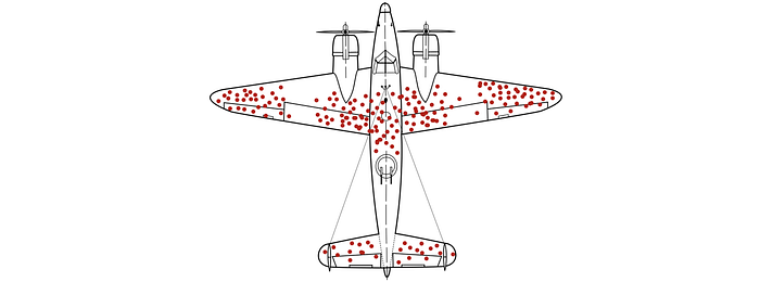
In World War II, the US military studied the most-hit areas of the plane that needed additional armor. This is vulnerable to survivor bias because the most important planes that we should study were lost in the fighting and never studied.
Survivor bias has another interesting definition. In some analyses, we include high-visibility data only and overlook low visibility data. Bill Gates and Steve Jobs dropped out of college and became very successful. Should we follow suit? Or is it just a rare high-visibility case? We oversimplify the analysis and use high-visibility data for our arguments. But, this is not necessarily intentional. For example, everyone wins in the stock market because whenever we win we broadcast it, whenever we lose, we keep silent. The availability and visibility of data often create bias.
Reporting bias is an umbrella term reflecting the fact that only some outcomes are reported. The report of research findings may depend on the nature and direction of the results. For example, in Funding bias, researchers may tend to release partial studies or data to support the financial sponsor's interests. Jones et al compared the outcomes of randomized controlled clinical trials specified in registered protocols with those in subsequent peer-reviewed journal articles. As Jones said,
Among the studies providing detailed descriptions of these outcome discrepancies, a median of 13 % of trials introduced a new, unregistered outcome in the published manuscript.
It concludes that
Discrepancies between registered and published outcomes of clinical trials are common regardless of funding mechanism or the journals in which they are published.
Discrepancies are not necessarily intentional. Sometimes, they are contributed by what is usually published in a journal. For example, ‘positive’ results indicating an intervention works are likely to be published than ‘negative’ results. This is part of the Publication bias. Language, location, and citation bias also impact what may be published. Will an AI research paper with equations get published easier than one using an empirical approach only? (even when there is a strong dissociation between the equations and the corresponding experiments.)
Studies cited more frequently receive more visibility. Researchers noted that studies reporting positive, statistically significant findings were cited more often than studies with neutral or negative findings. This is the citation bias.
Volunteer bias, self-selection bias, non-response bias happens often on online surveys. In one study I experienced last year, the 3,000 responders in a survey are 10 years older than the general user population. These responders are less critical compared with their younger peers. Therefore, the study was biased. People have the choice of smoking and non-smoking. Therefore, the characters of the smoking group may be different from the non-smoking group. For example, they have different ages and professionals. In other cases, it is difficult for substance abuse or sexual behavior surveys to reach out to high-vulnerability groups or religious groups.
Pre-screening increases the chance of a poor representation of the population or discourages some groups from participating. It also risks selecting participants who share similar characteristics that may influence results.
Healthy person bias points out the situation in which people volunteering or responding to a health study may be more healthy. They may be more concerned about their health and are predisposed to follow medical advice. In another situation, if participants are collected from a workspace, it is likely that they are more active and healthy than the general population,
Membership bias happens when we classify subjects into different groups and draw conclusions from them. Florida has a higher mortality rate than California. Should we draw a conclusion that California is better? This is grossly simplified as Floridians are on average 5.5 years older than Californians. The average ages in these two groups are so different that it is not a fair comparison. We often see claims that people with profession A suffer from disease B more. As shown here, such labels can be misleading. If the members in two groups are basically different, conclusions based on membership are usually biased.
Selection bias can be triggered by accessibility. Younger generations use different communication channels and are harder to be reached using traditional methods like phones. In health studies, certain populations have better access to health care. Therefore, certain diagnosis may appear more frequently in certain populations even if it is not. This is diagnostic access bias as someone has better access to diagnostic tests.
In the 1990s, Marin County in California had reported some of the highest breast cancer rates. Many possibilities were studied including genetic since Marin had a predominantly white population. Ascertainment bias occurs when the way data was collected was more likely to include some members of a population than others. Marin county is highly vulnerable to this bias since the population is richer with better health care access when compared to others. In short, more women are screened with a higher frequency and more sensitive equipment. These incidents may be reported better as the breast cancer rate in the counter was heavily scrutinized. (The breast cancer rate in Marin county has dropped significantly and the previously high rate was likely contributed by many factors.)
Performance bias happens when one group of participants gets more attention from reseachers than another group. For example, the difference in care levels result in difficult group make it hard to conclude the effect of a drug, as opposed to level of care.
In Berkson bias (admission bias)/paradox, the knowledge of a risk factor may unexpectedly increase its odd to the corresponding disease. For example, doctors may admit persons exposed to certain risks more frequently. Hence, in a hospital-based case-control study, the proportion of patients having these factors is increased. This leads to a higher odds ratio for some exposures.
Neyman bias (incidence-prevalence bias) is where the dead and/or very well are erroneously excluded from a study. This may lower or increase the odds ratio. For example, hospitalized patients have a greater risk for disease than the general population. Therefore, in a hospital study linking smoking and chronic obstructive pulmonary disease (COPD), we may find a stronger association than the general public. Below is an opposite case where the odd may be lowered.
For example, a hospital-based case-control study of myocardial infarction and snow shoveling (the exposure of interest) would miss individuals who died in their driveways and thus never reached a hospital; this eventuality might greatly lower the odds. (Quote)
Let’s talk about unmasking bias. A medication may cause bleeding. When these people visit a doctor, they may receive an intensive examination including cancer testing. During these testings, a number of patients may find to have cancer. A statistical correlation may be identified, despite no real association between the medication and cancer. In fact, we may draw different conclusions to the generation population that takes the same medicine.
Confirmation bias happens when people look for or recall information that confirms their own prior beliefs. Or they disregard information that contradicts their belief. This triggers experimenters to keep or to discard information based on what they believe or diagnose. Confirmation bias happens frequently in engineers. Engineers are always under the clock with firefighting issues. Biased search and interpretation of information are common. I personally feel that to success in troubleshooting firefighting issues, the best approach is to prove yourself wrong, rather than proving yourself right.
Measurement Bias (Information Bias)
After we collect participants representing the population in interest, the second bias comes with how information or measurements will be extracted. This step will introduce measurement bias that originated from the observer, the participants, or the instruments.
Observer bias is a general group of biases from the observers during the observation and recording of information. In one example, the bias is originated from different observers using different standards in recording or labeling data. For instance, different cultures may perceive the orange color differently. Hence, observers should go through standard training on how data is measured or classified.
Expectation bias can occur for observers and participants. Researchers or observers may be unconsciously biased towards what they are expecting. An observer’s expectations about an outcome influence how data is recorded or interpreted. For example, a nurse may expect a certain normal value on blood pressure. So a slightly lower or higher blood pressure may round up to the normal value instead. An observer may expect positive results for patients taking the drug but not those taking the placebo. In another example, an observer may interpret and record an overweight participant's answers with a bias towards diabetes conditions. Participants introduce expectation bias also. For example, patients may feel instantly better when taking a clinical trial drug even though it is just a placebo. To avoid expectation bias, a double-blind study is used in which neither the participants nor the researcher or observer knows which treatment is received until the trial is over.
A demand characteristic is a subtle cue that makes participants aware of the purpose of the experiment. Experimenters may give hints to participants on particular outcome or behavior is expected, by accident or not. Therefore, participants will alter their responses to conform to expectations.
Response bias is an umbrella bias that influences a responder’s responses. That includes another umbrella bias called self-reporting bias. It happens when participants compose their own answers through questionnaires, surveys, or interviews. Often, their responses are not completely true or honest. For example, social desirability bias happens when participants answer questions following the common social belief, for example, some people may be unwilling to agree “consuming alcohol regularly is not good”. Another example is recall bias. Memory can be very selective. In answering questions regarding the past, the response is selective or may be false. A discredited paper on the MMR vaccine had created a lot of publicity 20 years ago. Researchers found that more parents recalled the start of their child’s autism happened after the MMR jab, more frequently prior to the publicity. In a case-control study, patients are more likely to recall exposure to risk factors than healthy persons even though it may not be the case. Self-serving bias reflects the problem that in their response, people take credit for positive outcomes, but blame outside for negative outcomes.
Another response bias is the acquiescence bias (agreement bias). Participant may behave like a “yea-saying” and agrees with the question more frequently. To address leading bias, we design questions and answers in a way that does not lead participants to choose a specific set of answers. And we have to be careful as some of the bias may be triggered by questions asked previously in the survey. Courtesy bias happens when the participants do not fully state their dislike out of courtesy. Sometimes, they do not want to offend the person or the company they are responding to.
People behave differently when under watch. In Attention bias (Hawthorn effect), the participants’ behavior change causes inaccuracy in the conclusion. Between 1924 and 1927, a study was done at Hawthorne Works on whether lighting changes increase productivity. The story was usually told that being watched increases the productivity, not the lighting changes, (note: there were disputes on what the original findings should be.)
Other bias in clinical research
Let’s go through a few biases that happen in clinical research. In verification bias, it applies different rules on further verification. For example, if people test positive with the first test, they may go through a more accurate and thorough second test while others will just go through a simpler verification. The less complex method may capture fewer cases that lead to verification bias.
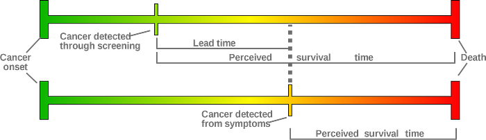
Badgwel et al studied the breast cancer survival rate for women 80 or older with or without regular mammography screening. They reported that the breast cancer-specific 5-year survival was 82% among women not screened, 88% among women with irregular, and 94% among regular users of screening. So screening improved the survival rate. Berry et al argue that it is biased by lead-time bias. The perceived survival time does not reflect the cancer onset time. The diagram below shows that two women can have the same cancer onset time but with different perceived survival times. The woman with screening has a longer perceived survival time because the tumor is detected earlier only. The survival time measured from both groups has a different standard (meaning).
Kamber et al reported a 66% reduction in mortality among patients with HZ after ACST treatment compared with patients without HZ after ASCT. (Don’t worry about these medical terms now.) But the study is likely biased by the immortal time bias.

There is a gap (immortal time) between the ACST treatment and herpes zoster (HZ) in the first case above. Let say a person dies before this immortal time (the second case) but he/she will have HZ if he/she does not die. But this case will be counted as a patient without HZ since the person dies before detecting it. This creates bias.
Similar bias may occur if we want to study the effect of a drug, for example, the effectiveness of a drug in avoiding readmission. In this example, a patient is released from a hospital and admitted into a study immediately. Say he/she will have a follow-up visit weeks later and a drug is subscribed to avoid hospital re-admission. However, some patients may readmit to the hospital before the immortal time (the gap between the hospital release and the drug subscription). Intuitively, the gap allows more healthy patients to join the “drug-treated” group. This bias will give a more favorable recommendation to the drug. Basically, the patient characters of these groups are different resulting in biased comparison.
Misclassification bias happens when a participant is categorized into the wrong group. For example, diseased individuals are classified as non-diseased and vice versa.
In a long trial, Chronological bias happens when participants are recruited at different times. Time is now another variable that influences the result greatly. The participants recruited can be different from those later. There are other changes that can happen. New measurement standards may be used and medical treatment has changed.
Detection bias happens when some group of population is underdiagnosed. For obese people, diagnosing prostate cancer via biopsy is more difficult and less accurate. Therefore, it underestimates the association of obesity with non-aggressive PCa.
Obesity is associated with risk of aggressive prostate cancer, but not with over-all PCa risk. However, obese men have larger prostates which may lower biopsy accuracy and cause a systematic bias toward the null in epidemiologic studies of over-all risk. (Quote)
If a specific professional find out one of the chemicals they have been exposed to is a carcinogen, those people may perform a cancer screening earlier than a non-exposed population. This is diagnostic suspicion bias.
This bias can be caused by prejudice. As quoted in the paper,
Findings reveal a clear and pervasive pattern wherein African American/Black consumers show a rate of on average three to four higher than Euro-American/White consumers.
As suggested by the paper, racial prejudice may be a factor in such discrepancy.
Understandably, when considering racial bias in diagnostic disparities, one would likely presume that clinician race would interfere with clinical judgment leading to diagnostic prejudice
Spectrum bias happens when the performance of a diagnostic test may vary in different clinical settings, i.e. the sensitivity (how good in spotting positive) and specificity (how good in spotting negative) of diagnostic tests vary in different settings. In theory, the same test used in a general doctor's office or a specialist office should have the same sensitivity and specificity. But empirical data may show discrepancies in factors like whether it is done in primary care, emergency care, or hospital. The largest overestimation happens in studies that included severe cases or healthy controls. Severe cases are easier to detect which would increase the estimated sensitivity. On the other hand, healthy controls overestimate the specificity.
Clinical research has one of the most detailed studies on the bias. For now, we will move on to other topics.
Confounder
In clinical research, the association between exposure and outcome can be distorted if there is a confounder.

Let’s introduce an example (original source) to explain the concept. A cohort study was done to associate obesity (BMI > 30) with cardiovascular disease. Data were collected for participants between the ages of 35 and 65 that are initially free of cardiovascular disease (CVD). They were followed over ten years to create the findings below.
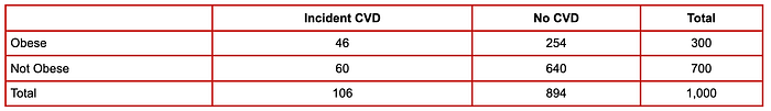
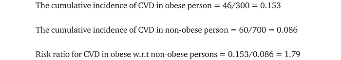
This suggests obese persons are 1.79 times more likely to develop CVD. However, age can influence both obesity and CVD as shown below. For people age 50+, there is a 0.5 chance of obesity while it is 0.17 for younger people. And older participants were more likely to develop CVD (0.1625) versus younger persons (0.075). Therefore, age is a confounding factor as it increases both the likelihood of obesity and CVD.

If the obese group in the study is older than the non-obese group, part of the increased CVD risk is originated from age. Therefore, the previous estimate of the association between obesity and CVD should be reversed down.
Engineers are trained vigorously on reasoning. Again, I personally found deadlines and firefighting often bring them to premature conclusions. Frequently, we create a causality relation between two factors that are actually independent of others. The failure to understand a third variable Z below can cost us a lot. Instead of fixing Z, we put focus on fixing X.

Susceptibility bias mistakenly associates factors that are related to A to another factor B when A is strongly associated with B. For example, patients with disease A may receive certain treatment T or medicine frequently. If disease A may also lead to disease B, we may associate the treatment T with disease B incorrectly even they are not related.
Collider bias.
Collider bias creates a distorted association in the opposite direction.
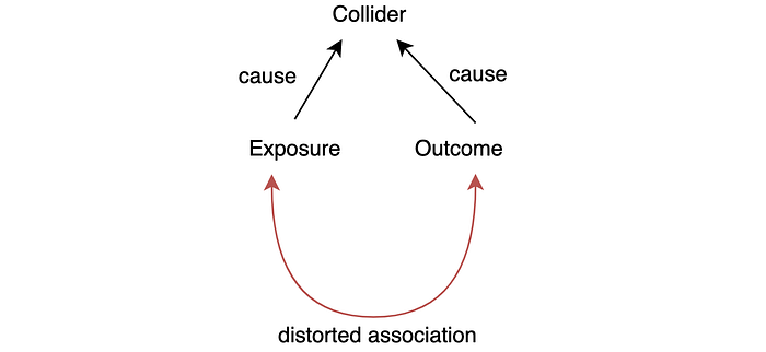
Are the locomotor disease and the respiratory disease related? It is pausable because the lack of activity may cause respiratory problems. One hospital study showed such a strong relationship. But Sackett found that they are not associated. The study is done with patients admitted to hospitals. Since both diseases can cause hospitalization, hospitalization becomes the collider factor. An unusual high coincident may happen for people hospitalized. As confirmed by Sackett, both are not related in a general population study.
In this example, locomotor disease and respiratory disease are independent of others. But if an experiment can control a collider, a distorted association arises. The hospital study controls all the participants to be hospitalized patients, therefore the study is biased.
This comes to a common theme in this article on the failure of identifying variables in the experiments that can impact outcomes. A general statement like A implies B can be misleading if there is another factor C that can impact A or B. In many engineering troubleshooting, we can waste too much time fixing A instead of fixing C.
Simpson’s paradox
Here is an example of what obvious right is wrong. A company with online and physical stores is doing a customer satisfaction study. As shown, the physical store is doing better so we may focus on how to improve the online store experience.
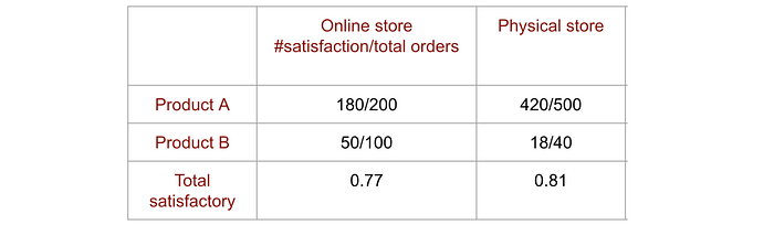
But the online store manager draws another conclusion showing every product has higher satisfaction in the online store than the physical store (for simplicity, we just show 2 products here). So who is right?
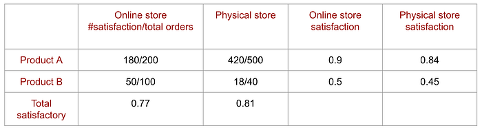
In the first report, we ignore the product variable and focus on the aggregated satisfaction ratio. It ignores the impact on product offerings. The lower rating in the online store is caused by the ratio of products sold. In a nutshell, product B has a lower satisfactory rating and customers buy more of them online. So we should look into why product B is more popular online and can we find better alternatives for product B. This example demonstrates the danger of oversimplifying the model with aggregated data, or what we measured.
In statistics, omitted-variable bias happens when a model leaves out one or more relevant variables.
Here was a real-life example studying the admission rate in UC Berkeley graduate school admission rate in 1973. As shown below, women had a lower admission rate compared with men.
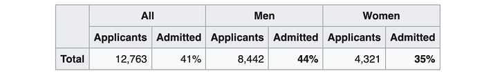
But if the data were analyzed at the department level, it showed a small but statistically significant bias in favor of women instead.
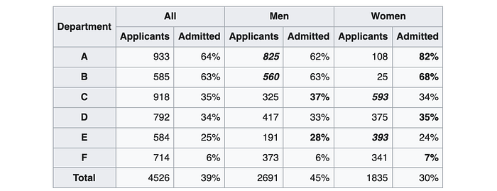
As concluded by the study,
The graduate departments that are easier to enter tend to be those that require more mathematics in the undergraduate preparatory curriculum. The bias in the aggregated data stems not from any pattern of discrimination on the part of admissions committees, which seem quite fair on the whole, but apparently from prior screening at earlier levels of the educational system. Women are shunted by their socialization and education toward fields of graduate study that are generally more crowded, less productive of completed degrees, and less well funded, and that frequently offer poorer professional employment prospects.
In short, women applied to departments that have lower admission rates.
Bias in Assignment
Allocation bias happens when researchers don’t use an appropriate randomization method to assign participants to different study groups and control groups. This is particularly problematic if the researchers can predict which group a participant may land into. This influences how they approach eligible participants and select candidates that have more positive outcomes for a particular group.
Channeling bias is a form of allocation bias, here is the explanation (the original)
Channeling is a form of allocation bias, where drugs with similar therapeutic indications are prescribed to groups of patients with prognostic differences. Claimed advantages of a new drug may channel it to patients with special pre-existing morbidity, with the consequence that disease states can be incorrectly attributed to use of the drug.
In a well-designed experiment, it is important that participants assigned to different study groups have no pre-existing differences. Otherwise, it will create a bias if we compare their results together. Let’s study the effectiveness of a training program. A test was given to two groups, one with the training and one without the training, to study which group performs better. If the company does not randomly assign employees to the training, pre-existing conditions may occur. For example, people who sign up for a class themselves may be more self-motivated. Or they may already know the subject matter better. So if we compare the test result on employees attending or not attending the class, there are pre-existing differences. The effectiveness of the class may be overstated.
Let’s discuss another example. For people that already visited a site a couple of times, we may display a new marketing campaign to them. Here, we want to study the effectiveness of this campaign. Very often, we compare the subscription rate of those visitors from the general visitors. This is biased. The first group visits the sites already and may show a stronger interest in the membership regardless of the campaign. So the campaign effectiveness may be overstated.
Next
In the next article, we will look into the technical side of AI biases.
