Caveats & Limitations on AI Fairness Approaches

In the last article, we discuss different AI fairness approaches that are commonly used. Unfortunately, they have plenty of weaknesses. We need to understand them carefully. Otherwise, we may do more harm than benefits. We will also look at the dilemma of these statistical fairness criteria approaches. Eventually, we will lead to a conclusion that while these are good methods to identify unfairness, they cannot certify it.
Dilemma on Fairness (A case study on COMPAS)
COMPAS is a decision support tool used by some U.S. justice systems. Judges and parole officers use the system to score criminal defendants’ likelihood of reoffending if released. It provides suggestions on bail, sentencing, and parole (a previous discussion). No ML fairness discussion will be complete without discussing it.
First, what are the objectives? And how do we frame the problem technically? We want to have maximum public safety with zero biases. The public wants safety while releasing as many defendants as possible.
In some cases, black defendants are substantially more likely than white defendants to be incorrectly classifed as high risk. To mitigate such disparities, several techniques have recently been proposed to achieve algorithmic fairness. Here we reformulate algorithmic fairness as constrained optimization: the objective is to maximize public safety while satisfying formal fairness constraints designed to reduce racial disparities. (Quote)
But in general, it is not possible to provide the most optimal solution in safety and fairness simultaneously. Both objectives have different optimal solutions. We need tradeoffs between them to achieve what we want.
We further show that the optimal unconstrained algorithm requires applying a single, uniform threshold to all defendants. The unconstrained algorithm thus maximizes public safety while also satisfying one important understanding of equality: that all individuals are held to the same standard, irrespective of race. Because the optimal constrained and unconstrained algorithms generally differ, there is tension between improving public safety and satisfying prevailing notions of algorithmic fairness. (Quote)
COMPAS tool addresses public safety. Yet, for credibility, it needs a general-recognized approach in fairness. In the Northpointe (COMPAS maker) defense to ProPublica, it states that scores are calibrated by group. Calibrated score achieves predictive parity. The chances of reoffending if released are the same in all the positive predictions for all groups. That is what COMPAS optimized for fairness.
With that, judges do not need to recalibrate the score based on race again. They can use it as-is for the risk factor without further account of the race. i.e. the scores are sufficient enough to make decisions without any other consideration. But it will not reconcile with the condition that both groups have a similar false positive rate. As black defendants have a higher re-offend rate if released, the higher false positive rate is unavoidable in this case.
By examining data from Broward County, Florida, we show that this trade-off can be large in practice. (Quote)
For sensitive applications, it remains elusive what are the best fairness criteria. How should we balance and tradeoff conflicting objectives? One of the disagreements is the role of social structural problems in making any fairness and design choices. Should such applications address those issues? Or this is a social issue that is beyond the scope of what the app should do. What should be addressed and how should it be addressed remain a political discussion rather than a technical one. For the rest of this article, we will focus on the technical side.
Caveats & Limitations on Statistical Fairness Criteria
Let’s look into the details of the Flordia Broward County data for COMPAS to explore the limitations and tradeoffs of statistical fairness criteria.
Here are the notations: x is the information of a defendant. Y is the outcome on whether the defendant will recommit a crime if released. R is the score from the model.
Outcome test
To achieve equal treatment, the same threshold has to be used to grant bail to two different groups. In the diagram below, the reoffence rate P(Y|X) for released defendants in each group is the mean of the distribution below the threshold. Since the blue group has a higher concentration of defendants with lower risk, its average reoffence rate is also lower.

So even the outcome tests may suggest discrimination towards whites, it is a premature conclusion.

Judges will release low-risk defenders regardless of the race. The outcome disparities are contributed directly by the distribution disparities of the low-risk defendants in each group. The real reason behind such disparities is not necessarily caused by racial bias. Raising such concern is premature. The question to ask is whether “race causes someone to be detained even though they should be on bail”. We need to hold other factors constant and verify whether the decision will be changed based on race.
Fairness Concerns
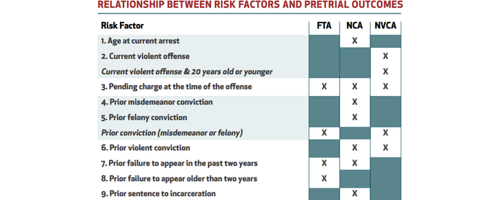
Next, we will follow the fairness concerns discussed in this talk. The talk finds ways to improve fairness but at the same time explains some of the limitations.
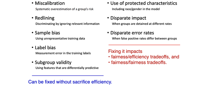
The diagram below is its eight fairness concerns. With careful execution, the concerns on the left can be addressed without sacrificing the main objective of the system. No public safety will be compromised. The fixes may not be easy but there are no side effects or controversy. But on the right, the fixes require tradeoffs between fairness and efficiency. This creates controversy on whether we trade one problem with another.
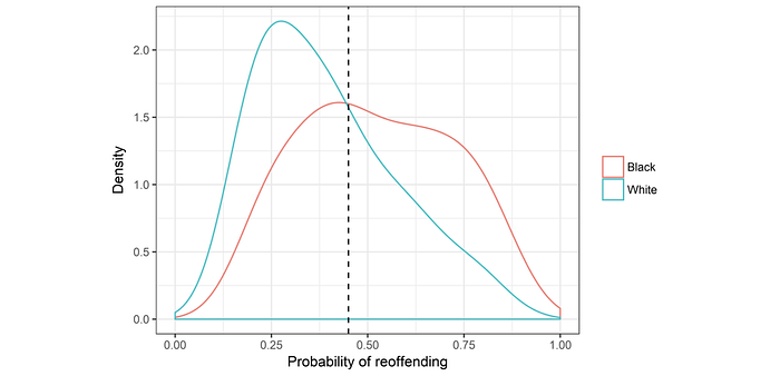
Miscalibration
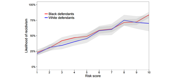
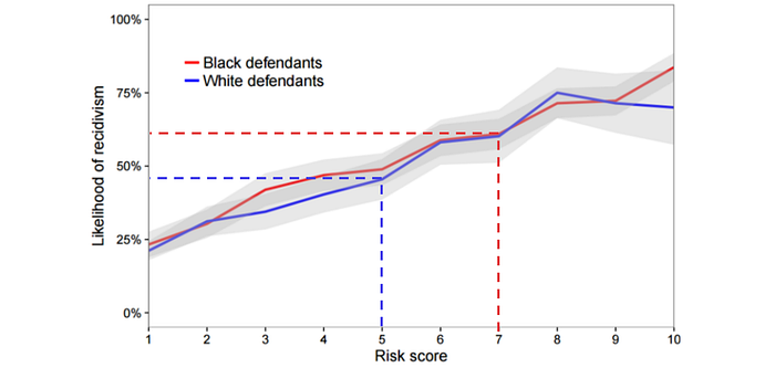
Miscalibration systematically overestimates the risk of a group. Here was an analysis done in 2017. The diagram below showed the relationship between the risk score and the likelihood of reoffending in COMPAS for black and white defendants. These scores were pretty calibrated by race. The corresponding scores indicate a similar likelihood of reoffending if released.
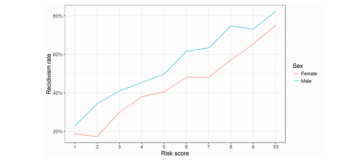
But another analysis showed that it was not true for genders. If judged by the scores, females could be detained unnecessarily more in Broward County than males.
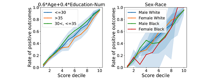
However, calibration may not be fair if we divide the group further (paper). In the diagram below, Group A and B are calibrated. Say, both of them have 3 defenders whose bails are denied. But the calibrations can cause violations or even more violations at the subgroup level. As an illustration, all of them may come from subgroups A1 and B2 only. In these subgroups, they are biased.

Hence, verifying bias with combinations of different attributes is important.
For simplicity, we will not cover possible resolutions. Please refer to these papers (1, 2).
Redlining
Redlining is another discrimination by ignoring relevant information about certain groups. Such omissions will cause biases in certain groups.
In lending, redlining is a form of systematic discrimination based on location, particularly in minority neighborhoods. In the process, it ignores an individual’s qualifications and creditworthiness. We will show an example that the scores are calibrated by group but yet, a particular group is discriminated against.
Let’s consider the creditworthiness of location A and location B below that are exactly the same.
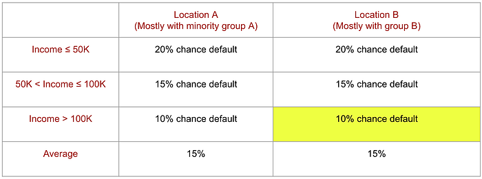
We can recalibrate all the default scores in location A by replacing them with the group average. i.e. for location A, everyone has a default score of 0.15. Ironically, the new scores remain calibrated. Calibration by group requires

People mistake that it means P(Y=1) = r for everyone scoring r, i.e. if a person score 0.15, P(Y=1) = 0.15 for the individual. That is not true.
Let’s say group A has only three people with scores of 0.13, 0.15, and 0.17 respectively. Their average is 0.15. We can recalibrate all their score to 0.15 and it will still meet the requirement on calibrated by group, which only requires the set of people scoring 0.15 to have an average of P(Y=1) = 0.15. Calibration by group is about statistics on a group but not on an individual.
To discriminate Group A, we just accept loans that have a possible default score of no more than 0.1. All people in location A will not get a loan. Effectively, we discriminate against the minority Group A.
In general, we do not have to replace every score with the average. In the example below, we can simply squeeze the score distribution from the black curve to the red one below. As long as we pair people smartly to maintain a specific average at each score, the scores can remain calibrated. In the red curve below, the new calibrated scores will put everyone below a threshold. If this is a credit score, we manage to fail everyone in this group.
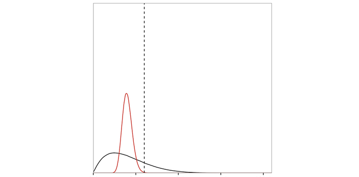
This leads to an important limitation on calibration. In ML, we can penalize the violation of calibration by group in the objective function. Yet, even the criteria are met, there is no guarantee on what the model learns. Indeed, it may just replicate how we can cheat.
Calibration is necessary but not sufficient for fairness.
Since it is not sufficient, the proof is not complete. This single criterion is necessary but not sufficient for fairness. Using it as single support evidence in a fairness certification is flawed. In short, it is a good mechanism to spot unfairness but it cannot certify fairness.
Aggregated data can lead to poor conclusions, in particular, if the variable that averaged out holds critical information for individuals. In real life, stereotypes loss the individual information that matters.
Another lesson is we cannot determine the fairness of an algorithm without inspecting all the information. This holds against the belief that sensitive characters should be eliminated from the input of a model. The key difference is whether we can use the information correctly without the bias context.
Sample bias
Sample bias happens when the samples collected do not represent the population in interest. Predictive policing algorithms may over-focus on certain neighbors and ignore others. This focus may result in further scrutiny that results in a higher reporting rate. Other neighbors with less scrutiny will be underreported. So the algorithms will give further attention to areas under scrutiny. This creates a self-reinforcing loop that keeps bias happening. Understanding this feedback loop is important. From my own professional experience, many ML models, like recommender, are stuck in this loop! The question here is how can we balance exploitation with exploration. Are the collected data biased?
Label Bias
Label bias is about measuring errors in the label. A predictive policing algorithm wants to predict crimes. Crime rate is the outcome (label) that we are interested in. But we often mistake that the crime rate is the same as the arrest rate. If minority group areas are under heavy scrutiny, there will be an overreporting of less serious arrests while other areas are underreporting. Therefore, this proxy measure does not reflect the true crime rate and it can be highly biased against minority groups. To measure the crime rate, a more reliable proxy measurement is needed. From criminologists, the chance of being arrested is about the same in any race for serious crimes. Therefore, the serious crime arrest would be a better proxy since the chance of reporting will be more balanced.
Subgroup validity
While the accuracy in the labels can cause bias, the accuracy in input features can have similar problems. For example, if the number of arrests is used as an input feature, we already show that it can be significantly biased in minority groups. This feature is less predictive for future outcomes. For fairness, we need to evaluate how good a feature is in making predictions for each group. We should mitigate disparity in feature performance in making predictions.
Use of Protected Characters
Equal treatment assumes the outcome should be completely irrelevant to a sensitive character. In real life, a correlation usually exists. It may be wholly or simply partly caused by bias. Nevertheless, if we remove the protected characters, we will remove the non-bias aspect also. This creates an incomplete model that leads to a sub-optimal solution.
In ML, we can create a causal model (a graphic model) listing the possible paths on how a decision is made. With massive data, we can train the model to learn both biased and non-biased aspects of these sensitive characters. In making decisions, we can remove the biased portion so we can make a fair and optimal decision. In a later example, we will elaborate this concept further with a study in the UC Berkeley admission.
In other cases, if bias is detected, we can create group-specific thresholds to rebalance the issue. This reestablishes equal outcomes. As discussed in these research papers [1, 2, 3], new technologies open up possibilities of using protected characters for equal outcome.
The caveat is we know the use of protected characters can be beneficial in creating a fairer model if it is done correctly. Again, current US anti-discrimination laws do not allow it in protected domains.
Disparate impact
In disparate impact, we compare the statistical disparity between groups to identify biases. While this is an effective method to locate potential bias, statistical disparities may draw us to the wrong conclusion.
College students eat more healthily compared with other professionals. They have low BMI (body mass index), heart disease, and diabetes rates. We know this is not true. Students eat junk food, Why does the evidence draw the wrong conclusion? College students have very different characters compared with other professionals. They are much younger. Their low BMI index is related to age. The comparisons between groups are not apple-to-apple.
In the Broward county data, black defendants had been deemed a higher risk of committing a crime. But we need to ask that do the black defendants and white defendants have similar characters.

In fact, there are many risk factors. For example, do the defendants have the same age distributions? Will these disparities result in different risk levels?
This is called membership bias which happens when we compare groups that have different characters.
To look deeper into the possible bias, we need to go deeper to eliminate as many differences as possible. For example, if there is no statistical disparity in different age groups with the same number of convictions in both races, the hypothesis on the racial bias will be less likely.
Disparate error rates
Similar problems happen in disparate error rates also.

ProPublica mainly argued that COMPAS was racially biased because of the much high false positive rate in black defendants. Again, this was caused by different risk distributions in both groups.
Even groups may have the same average risk, different shapes (variance) result in disparate statistics.
Once a threshold is chosen, we are looking at sub-segments of both groups rather than both groups. This can lead to disparate detention rates and disparate false negative rates. The samples are no longer representable for the general populations in interest. Any generalized statements can be misleading.
Optimal solutions
People want to maximize public safety with the smallest possible number of detainees. This paper claims that the most optimal unconstrained algorithm, without fairness consideration, should apply a single and uniform threshold to all individuals, irrespective of a group membership.
To take group fairness into consideration, we can add fairness equality to the optimization problem as a constraint. The same paper proves that the optimal constrained algorithm for equal detention or false negative rate requires race-specific thresholds. This demonstrates tensions between group fairness and individual fairness, i.e. the optimal solutions are different and group fairness will achieve at the cost of individual fairness. As shown below, the optimal constrained algorithm would apply a lower threshold to detain white defendants in Broward County.
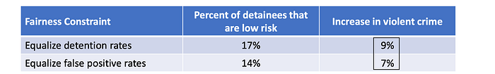
Regardless of whether we are equalizing detention rates or equalizing false positives rates, more lower-risk defendants will be detained because of their race. These victims can raise a 14th amendment case on the equal protection clause.

These criteria will also raise the violent crime rates. Some higher-risk defenders are now released.
Since this will happen in minority neighbors more often, these neighbors can suit for the 14th amendment because of the crime rate increase due to race-based decisions.
False positive rate (FPR)
Can we achieve the same FPR for different groups without achieving fairness?
Let’s consider two different cases below. According to the Broward County data, there are disparities in FPR. But say the policy chief arrests more jaywalkers in the orange group’s neighborhood, the FPR for the orange group will be reduced as these jaywalkers increase the negative pool (the denominator for FPR).

The algorithm has not changed so as the decisions. We do not make the algorithm “fairer”. But the disparity disappears.

Here is a good example that without examining the details of the data, statistical data may not give us the complete picture. And it is vulnerable to cheating and manipulation.
Limitations on Statistical Fairness Criteria
This leads us to a more general topic in understanding the limitation on statistical fairness criteria.
Mutual exclusive of fairness criteria
As discussed before, there are 3 major fairness criteria.
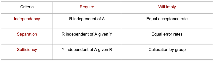
Unfortunately, any two of these criteria can be proven to be mutually exclusive in general, i.e. we cannot have a solution satisfy both criteria at the same time.
Let’s prove one of them. First, we assume A and Y are correlated. If sufficiency (Y⊥A | R) holds, then A ⊥ R (independency) will not hold.

For simplicity, please refer to this talk for other proof.
Statistical Fairness Criteria
As discussed before, many claims like “Group A has a much higher negative false rate” can suffer membership bias badly. Different groups have very different distributions of their characters. For example, one group may be younger or healthier in a healthcare study. We may not compare apple to apple. Even they have the same mean of a character (say, same average risk), the shape of the distribution can still lead to different statistical disparities.
Another key limitation of these statistical criteria is that they are observational. The data can be biased, cheated, or manipulated. Statistical data is a passive observation. As shown before, to avoid wrong conclusions, we need to look into data in detail and examine how it is collected and measured. In short, we need to take it apart. Without creating scenarios, we cannot prove or disprove the conclusion scientifically. These constraints lead to significant limitations.
Interventions
Interventions create scenarios to see how a model performs. In intervention, we substitute a sensitive character A by a specific value, say do(A=a) set all A to a. Below, we evaluate the impact on R for different substitutions. In doing so, we discover any disparity if we force one value over another.

But this may not be feasible in many real-life problems. As illustrated by this paper,
The notion of an “effect of race” is ambiguous: the effects may vary depending on what is meant by race. It may include skin color and its perception by others, parental skin color and its perception by others, cultural context, or genetic background — all considered separately or jointly.
In short, we cannot just change the race information from black to white.
Hence, in some problems, a better alternative is to consider proxies instead of sensitive attributes. Intervention based on proxy variables seems to be more manageable. And detailed proxy interventions will be discussed in these papers (1, 2). This process involves the modeling of a casual model. However, we will not elaborate on it further. Instead, we will demonstrate the casual model concept with a later article on counterfactual fairness instead.
Statistical Criteria is observational
This discussion leads to a more generic issue. Let's define a criterion as observational if it is a property of the joint distribution of input feature X, group A, classifier C, and outcome Y. True positive rate is observational since it is derived from this joint distribution. In short, any observational criteria is just a probability statement involving X, A, C, Y. (details)
To demonstrate the limitation on observational criteria, let’s consider two scenarios with different fairness approaches. If they both have identical joint distributions, their statistics will be the same. Hene, these statistics cannot distinguish these scenarios and cannot be a good judge in certifying what is better.
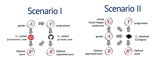
In the computer industry, there are more male programmers than female programmers. The two different systems above score candidates for a programmer application. In these scenarios, the joint distribution of A, X, and Y are the same. We are dealing with the same group of population. In scenario 1, the optimal score is derived from information on whether a person visited Pinterest and Github. It takes advantage of the positive and negative factors for maximum predictability. (As these two sites will be visited more by one gender.) For the optimal separated score (optimal decisions with fairness constraints), it does not use Pinterest because this information can derive the sensitive character (gender). It violates equal treatment. The Github information is acceptable because the casual model is trained in the way that X₁ can be derived by Y (a programmer). Y is sufficient for X₁. Given Y, X₁, and A are independent. In scenario 2, it uses a different fairness approach. The optimal separated score will take advantage of the gender information directly to create an equal outcome for both genders. For the optimal score, it only uses the factor of whether a candidate has a CS degree. Both scenarios have very different fairness approaches but yet they have the same joint distribution. Hence, any observation statistics drawn from the joint distribution cannot distinct both scenarios.
This comes to a very important insight in this article:
Statistical fairness alone cannot be a certificate of fairness. It should be a tool to locate suspicious bias but not necessarily a proof of fairness.
In addition, we need to be very careful on whether to use these fairness metrics as part of an objective function. We have to ask if those statistic criteria are met, what we really achieve underneath. As shown before, what we get is not really what we think sometimes. It can give us the impression that it is fair when it is not.
What is Biased and What is Not
In 1973, a UC Berkeley study evaluated whether its graduate admission was gender-biased. Statistically, women were rejected more often than men.
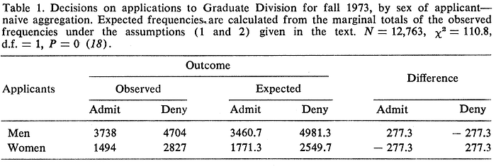
Here is the abstract of the paper. It demonstrated that women had a lower admission rate but it was not because of gender bias.
Examination of aggregate data on graduate admissions to the University of California, Berkeley, for fall 1973 shows a clear but misleading pattern of bias against female applicants. Examination of the disaggregated data reveals few decision-making units that show statistically significant departures from expected frequencies of female admissions, and about as many units appear to favor women as to favor men. If the data are properly pooled, taking into account the autonomy of departmental decision making, thus correcting for the tendency of women to apply to graduate departments that are more difficult for applicants of either sex to enter, there is a small but statistically significant bias in favor of women. The graduate departments that are easier to enter tend to be those that require more mathematics in the undergraduate preparatory curriculum. The bias in the aggregated data stems not from any pattern of discrimination on the part of admissions committees, which seem quite fair on the whole, but apparently from prior screening at earlier levels of the educational system. Women are shunted by their socialization and education toward fields of graduate study that are generally more crowded, less productive of completed degrees, and less well funded, and that frequently offer poorer professional employment prospects.
In UC Berkeley, the admission rates for women were higher than men in many departments. It was the opposite of the general admission rate.

So what was the problem? The average rate depended on the women's application rate for the department i.
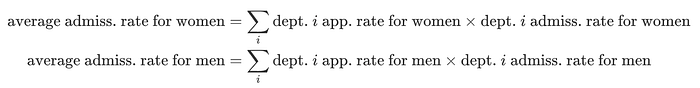
If women applied to departments with low admission rates more, they could have a lower admission rate even though it was the opposite in each department. In the example below, both departments accept women more. Yet the general acceptance rate for women is lower because they apply to departments with much lower acceptance rates. In many probability problems, we often neglect the frequency of the event i. This is a major mistake!

This case study demonstrated that not all factors that look biased are biased.
Active researches are done in developing casual models such that we can quantify the biased and non-biased context of the gender better. Gender can influence admission as an unfair bias. But admission can be influenced by the department that women choose.
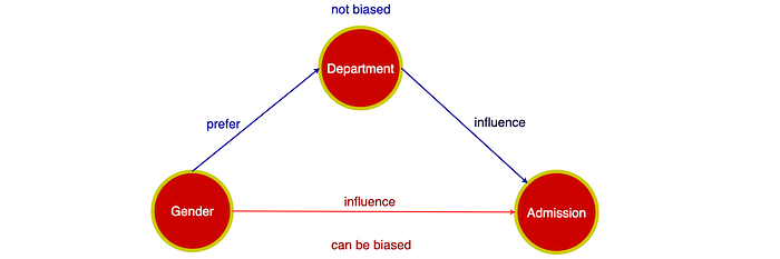
For decision-makers, we can just eliminate the biased path from the model in making decisions. For example, we believe that gender should have not direct relevancy on the admission decisions. So the lower path should be eliminated. Completely ignoring gender in a model can be counterproductive. This concept is under active research. We will demonstrate the idea further in Counterfactual Fairness in another article.
However, designing a casual model requires a lot of assumptions — what components should be there and what are the dependency. As shown below, two designers may come with two very different models.
Case Study (Job Advertisements)
A previous study showed that the Facebook Ad recommender was gender-biased. This is a sensitive topic because gender discrimination is illegal in a job application and the US law covers job advertisements too.

In another paper, it introduces a hypothetical discrimination suit story to analyze the tensions on the anti-discrimination principles and their implications on the technical solutions.
In the paper, the application P(click) predict how likely a person will click on a particular advertisement. It uses the user click pattern and other user patterns to make predictions. It displays ads that a person is more likely to click. Suppose women are likely to click on ads for shorter-term service sector jobs and men are more likely on longer-term blue-collar jobs. Since the latter jobs may pay better, the Ads targeting strategy may contribute to income disparity.
Say, gender is an input feature to p(click). In the UK, the regulator will argue that this was direct discrimination because gender is used in deciding what Ads to display. P(click) agree not to input gender explicitly to the model. But in a separate statistic analysis, a user’s gender can still be predicted from other variables. The regulator argues that gender is still part of the decision, the proposed change still violates direct discrimination.
P(click) argues that well-calibrated ML models trained on representative datasets always reproduce patterns in the training data. Therefore, the predictions are correlated with group membership. P(click) shows that the correlation is because of the types of jobs each gender is more likely to click.
Because there are no direct correlations of using gender to the decisions, the regulator requests P(click) to explain the disparate outcome instead. It requests P(click) that there are no reasonable alternatives.
Therefore, P(click) decides to explore two alternatives. The first one introduces demographic parity. P(click) can require the average income of job ads displayed to both genders cannot have a 5% disparity. This solution will hurt revenue since less relevant ads may be displayed. Also, it reduces the chance for people to find their jobs. However, since both genders will use different standards for Ad display, it could violate the equal treatment principle.
The second option was to put gender information back. As the paper said,
Since p(click) was producing persistent disparities in the average income of job ads across gender, it was showing that gender is statistically relevant to predicting click probability. Including gender would enable the model to make more fine-grained predictions in full knowledge of underlying disparities, rather than being blinded to them. … experiments showed that including gender as a feature narrowed the disparities between the average income of job ads shown to men and women, although it did not eliminate them.
But again, the regulators may not like it as they rule before that it violated equal treatment.
Note: Anti-discrimination laws are domain-specific. (credit, employment, housing, education, housing, public accommodation, etc …) It does not cover every aspect of life. This example does not apply to other domains. But the discussion remains relevant.
Human v.s. Machines
While we discuss the complexity of fairness, we don’t want to create the impression that AI is evil.
AI systems, like humans, can be biased. But heavy spotlights on these systems may do no justice also. The biases in many ML deployments are not excusable. It should be fixed and it can. But studies, like the one about loan underwriting, demonstrate software systems can reduce bias significantly compared with decisions made by professionals. So even your mileage may vary, AI systems can bring significant improvements over manual processes if they are validated properly. As a solution provider, be prepared for scrutiny. The era of “see no evil, hear no evil” is over.
As stated in this paper, the improvement of prediction (a domain where ML focuses on) can improve public safety.

More accurately identifying high risk defendants in the New York data reduces crime rates by 25%, holding release rates constant, or reduces pre-trial jailing rates by over 40% with no increase in crime. … Importantly, such gains can be had while also significantly reducing the percentage of African-Americans and Hispanics in jail. (Quote)
