GAN — Energy based GAN (EBGAN) & Boundary Equilibrium GAN (BEGAN)
GAN is a minimax game in which opponents take action to undercut the other. This makes GAN much harder to converge, if it ever happens, than other deep learning models. As part of the GAN series, we look into EBGAN and BEGAN to see how we change the network design of the discriminator to address the stability problem.
Overview
We wish we know exactly what deep learning networks are learning, but in reality, there are many surprises. By chance, generating green grapes may be easier to fool a GAN discriminator. If this persists, the generator will generate green grapes only to reduce the generator cost. Now, the images fitting to the discriminator is biased. The discriminator will specialize in detecting green grapes and neglect others. But the story does not end here. The generator will counteract by shifting to another color. This model will never converge as it engages in such a never-ending cat-and-mouse game.
This explanation oversimplifies what happens in practice. But it illustrates one important point. The goal of the discriminator in the original GAN cost function is to beat the generator. However, this can be done by some greedy approaches that are penny wise but pound foolish. Energy based GAN (EBGAN) uses a different criteria.

Instead of designing a discriminator similar to a classifier, the discriminator uses an autoencoder which extracts latent features of the input image by an encoder and reconstruct it again with the decoder.

This discriminator outputs the reconstruction error (mean square error MSE) between the input image and the recreated image instead of a probability value in the original GAN.

Now, we need to convince you that this metric behaves like the probability D(X) used in the original GAN. In EBGAN, we use real images to train the autoencoder to reconstruct images. For a poorly generated image, the reconstruction has a very high error because it misses all the latent features needed by the decoder (that is why it is a poor image). If the generated image looks very real, its reconstruction cost will be low. Even it is less obvious, the reconstruction cost is an indirect but good metric to critic the generated images.
Next, we need to change our objective function so we can train the discriminator to be a good critic and a good autoencoder.
Objective function
To train the discriminator, its cost function composes of two goals:
- a good autoencoder: we want the reconstruction cost D(x) for real images to be low.
- a good critic: we want to penalize the discriminator if the reconstruction error for generated images drops below a value m.
For the generator, we want to lower the reconstruction error for the generated images. Here is the cost function for the discriminator and the generator.

D is the reconstruction loss and L is the loss function. Don’t confuse by them.
In the beginning, the reconstruction errors for generated and real images are high. The loss in the discriminator comes from the reconstruction loss of the real images since the hinge loss ([u]+) is zero. The discriminator concentrates on creating a good autoencoder for real images. In parallel, the generator learns from the reconstruction errors from the generated images to improve itself. This reconstruction error will gradually drop. Once, it falls below m, the discriminator will also focus on locating features that discriminate generated images. These criteria focus on extracting latent features of real images while locating what generated images are missing. It is less vulnerable to greedy optimizations that draw too much conclusion on a small set of features. To lower the cost of the discriminator, it needs to capture enough features to reconstruct real images.
Repelling regularizer
To avoid mode collapse, EBGAN-PT, a variant of EBGAN, adds an additional cost function for the generator. S is the feature output from the encoder for the generated images. We compute the pulling-away term (PT) which measures the cosine similarity among all generated images features S in a minibatch.

If the mode collapses, the feature vectors will be similar, i.e. the angles are close to zero and the cosine will max-out. Therefore, it will add a high penalty if there are too similar.
Boundary Equilibrium Generative Adversarial Networks (BEGAN)
Recall that, EBGAN uses the MSE to calculate the reconstruction errors D. The loss for the discriminator L is computed as:

In a generative model, we try to match the data distribution of generated images with the real images. BEGAN is based on a proposition that matching the reconstruction loss distribution of real images and generated images lead to the matching of the data distribution of real images and generated images.

In short, if we manage to match their reconstruction loss distribution, the generated images will have the same data distribution as real images. As a direct quote from the research paper:
This seems to confirm experimentally that matching loss distributions of the auto-encoder is an effective indirect method of matching data distributions
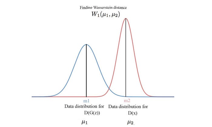
BEGAN has the same discriminator design to compute the reconstruction loss. But it changes the loss function L of the discriminator. The objective of the discriminator is to maximize the difference of the data distribution of the reconstruction losses of real images and generated images. While there are many methods including KL-divergence to measure the difference, BEGAN uses the Wasserstein distance. In a minibatch, we compute the reconstruction error for each real and generated image (same as EBGAN). The results form two data distributions one representing the reconstruction loss of real images and the other for the generated images.
Wasserstein distance W measures the effort to change from one distribution to another. The original equation is intractable. Hence, instead of explaining what is Wasserstein distance, we just show you how we can estimate it.

where m1, m2 are the means of the two distribution. i.e. the Wasserstein distance has a lower bound equal to the absolute difference of the means of the two distribution.

But instead of finding the means, we can just use the total reconstruction cost of real images and generated images in a mini-batch. Here is the new cost function.

Let’s change our notation to match with the one used in the BEGAN paper.

where L is the output of the autoencoder.
The loss function for the generator remains the same:

Imbalance
The loss function for the discriminator is similar to the EBGAN except that we skip the hinge function.

Their goals for the discriminators are the same: being a good autoencoder and a good critic. However, these goals may not be in-sync. A balance training without one being too far ahead of the other is often considered beneficial. Otherwise, we may overfit the discriminator or the generator and in the worst scenario, the mode collapses and never recover. Mathematically, we can express the balance point as:

And we change the objective function so we can rebalance one’s impact on the cost function if one is more optimal than the other:

Nevertheless, k is sensitive to the minibatch sample x. We don’t want it to fluctuate because of the data variation. To solve that, we use a running mean k during the course of the training. The following is the cost function with the running mean for k.

where λ (0.001 in the paper) is the learning rate of the running mean. You may challenge the reason to maintain k to be 1. Indeed, we introduce a hyperparameter γ and allow a slight bias of our goal to improve the image quality at the cost of diversity.

Finally, this is the cost function for BEGAN.

We initialize k to be zero at the beginning so it gives time to develop the autoencoder first.
We can experiment with the impact of γ by dropping its value from 1. As γ gets closer to 0, the discriminator will focus more on the autoencoder for better images than counteract the generator. So the generator start overfitting itself and the mode drops. So when we drop γ, the image quality improves but the mode starts collapsing too.
Model design
The network design for the autoencoder and the generator are shown as below. The design for the generator and the decoder is the same but they are not sharing the weights.

Model convergency
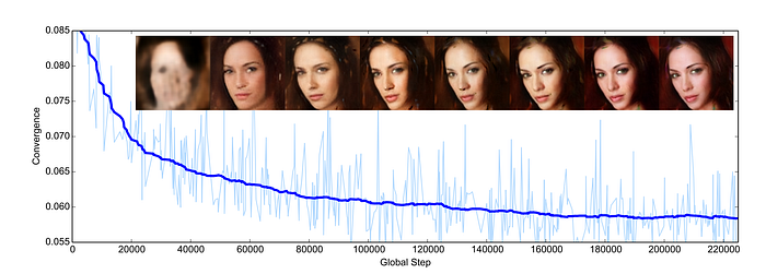
In GAN, the cost function is not a good measurement of convergency or image quality. GAN is a minimax game which sometimes you win and sometimes you loss. The cost value at a particular instance does not related to the image quality or the model convergency. In BEGAN, the image quality is indirectly related to L(x) of the real images. When the model converge, the difference between the reconstruction losses should converge to zero.
To monitor the model convergency, we can plot:


Experiment
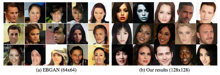
Compared with EBGAN, BEGAN can generate images with higher resolution and higher quality.

As γ drops, the image quality improves but we start seeing some pictures looks very close to other.

Here we vary the latent variable z and see how the generated images are changed. Here we see the changes are not random which indicate our models are learning rather than memorization.

