GAN — StyleGAN & StyleGAN2

Do you know your style? Most GAN models don’t. In particular, does the GAN model has more methodical ways of controlling the style of images generated? In the vanilla GAN, we generate an image from a latent factor z.

Usually, this latent factor z is sampled from a normal or uniformed distribution and contains factors that determine the type and the style of the content generated. (For those having problems following the discussion so far, please refer to this article first.)

With this in mind, we have two important questions asked:
- Why z is uniform or normal distributed?
- As z contains the meta-information, should it play a more dominant role in generating data in each convolution layer? (Rather than as an input to the first layer only.)
Note: throughout this article, we will use the term style when we refer to meta-information including type and style information.
Here are the generated images from StyleGAN2.

Latent Factor z
In general, machine learning (ML) loves its latent factors to be independent of others which makes model training easier. For example, height and weight are highly entangled (taller people weigh heavier). Therefore, the body mass index (BMI) that computed from height and weight is more regularly used regarding fatness. The required training model will be less complex. Unentangled factors also make the model easier to interpret correctly.
In GAN, the distribution of z should resemble the latent factor distribution of the real images. If we sample z with a normal or uniform distribution instead, an optimized model may require z to embed information beyond the type and style. For example, let’s generate portraits for military personnel and visualize the data distribution of the training dataset with two latent factors: masculinity and hair length. The missing upper left corner below indicates that male soldiers are not allowed to have long hair.
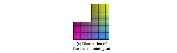
If we sample this space uniformly, the generator will try to reproduce portraits for male soldiers with long hair. This should fail because we don’t have any training data to learn it. From another perspective, when the normal or uniformed distribution is used for sampling, imagine what latent factors that the model will learn. Indeed, it will be likely far more entangle and complex that it should be. As the StyleGAN paper argued that “this leads to some degree of unavoidable entanglement”.
In logistic regression, we apply the change of basis to create a linear boundary in separating binary classes. In StyleGAN, it applies a deep network called the mapping network in converting the latent z into an intermediate latent space w.
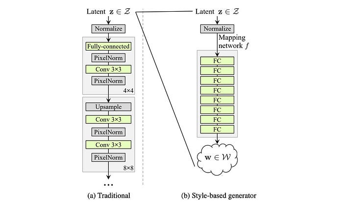
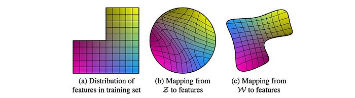
Conceptually, StyleGAN warps a space that can be sampled with a uniform or normal distribution (middle below) into the latent feature space (left) needed to generate the images easily. The goal of this mapping network is to create untangled features that are easy to render by the generator and avoid feature combinations that do not happen in the training dataset.
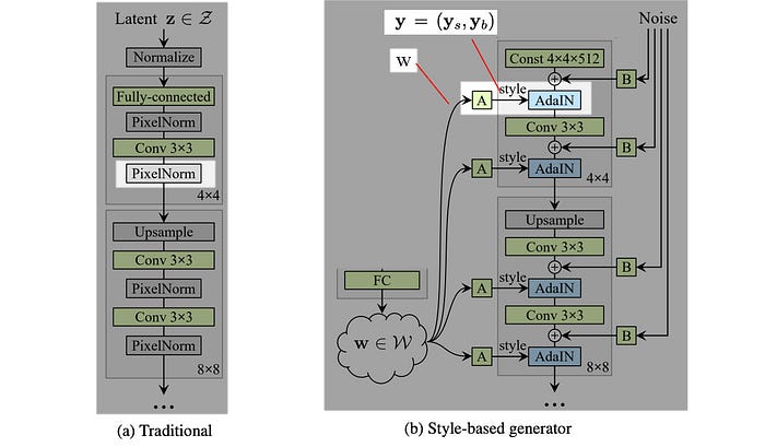
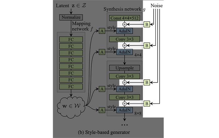
StyleGAN introduces the Mapping network f to transforms z into this intermediate latent space using eight fully-connected layers. w can be viewed as the new z (z’). Through this network, a 512-D latent space z is transformed into a 512-D intermediate latent space w.

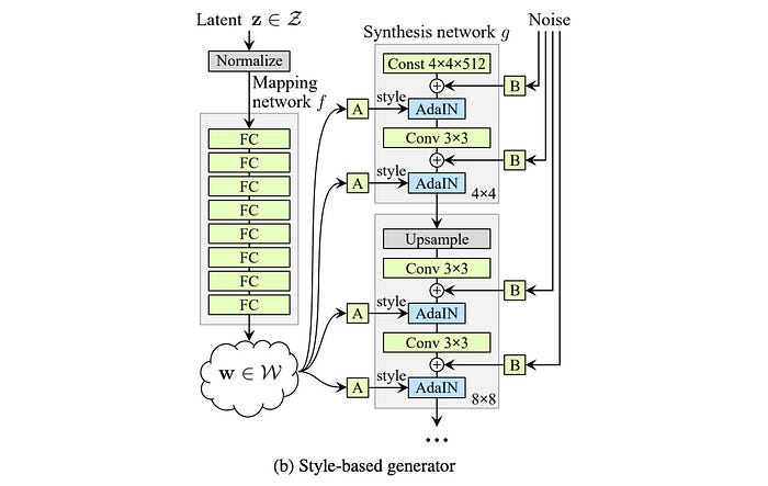
Style-based generator
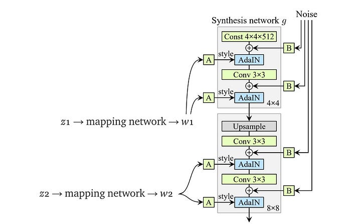
In the vanilla GAN, the latent factor z is used as the input to the first deep network layer only. We may argue that its role diminishes as we go deep into the deep network. In the style-based generator, we apply a separately learned affine operation A to transform w in each layer. This transformed w acts as the style information applied to the spatial data.
In the StyleGAN paper, it starts with the Progress GAN network design (details) and reuses many hyperparameters including those for the Adam optimizer. Then the researcher experiments with design changes to see whether the model performance is improved.
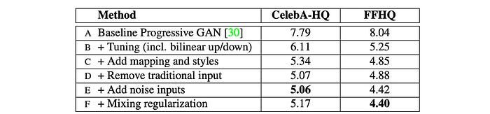
The first improvement (B) will be replacing the nearest-neighbor up/downsampling in both discriminator and generator networks with bilinear sampling. The hyperparameter will tune further and the model will also be trained longer.
The second improvement (C) will be the addition of the mapping network and the styling. For the latter part, the AdaIN (adaptive instance normalization) will replace the PixelNorm in applying styling to the spatial data.
AdaIN (adaptive instance normalization) is defined as:

where the input feature map is normalized with instance normalization first. Then, StyleGAN scales and biases each normalized spatial feature map by the style information. (μ and σ are the mean and the standard deviation of the input feature map xᵢ respectively.) In each layer, StyleGAN computes a pair of style values (y(s, i) and y(b, i)) as the scale and the bias from w to apply the style to the spatial feature map i. The normalized feature influences the amount of style applied to a spatial location.
In vanilla GAN, the input to the first layer is the latent factor z. Empirical results indicate no benefit in adding a variable input to the first layer of StyleGAN and therefore, it is replaced with a constant input. For the improvement (D), the input to the first layer is replaced by a learned constant matrix with dimension 4×4×512.
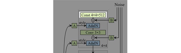
“Style” in the StyleGAN paper refers to major attributes of the data like pose, and identity. In improvement (E), SytleGAN introduces noise into the spatial data in creating stochastic variation.
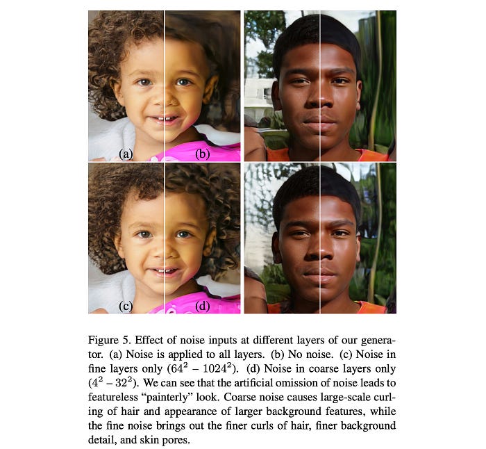
For example, the added noise is observed to create variants on the placement of hair (below), stubble, freckles, or skin pores in the experiments.

Say, for the 8×8 spatial layer, an 8 × 8 matrix is created with elements containing uncorrelated Gaussian noise. This matrix will be shared among all the feature maps. But StyleGAN will learn a separate scaling factor for each feature map and multiple it with the noise matrix before adding it to the output of the previous layer.
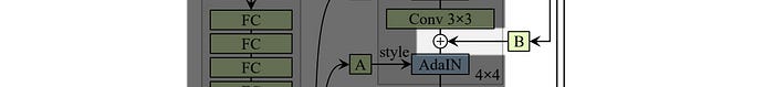
The noise creates rendering variants with benefits demonstrated below when compared to no noise or only applied to certain resolutions. The StyleGAN paper also suggests that it mitigates the repetitive patterns often seen in other GAN methods.
In short, style addresses key attributes of the images in which apply globally to a feature map. Noise introduces local changes in the pixel level and targets stochastic variation in generating local variants of features. (these claims are reinforced from observations)
Check out the next 60s in this video on how noise creates different image rendering.
The last improvement (E) is on Mixing regularization.
Style Mixing & Mixing regularization
Previously, we generate a latent factor z and use it as a single source in deriving the styles. With Mixing regularization, we switch to a different latent factor z₂ to derive the style after reaching a certain spatial resolution.
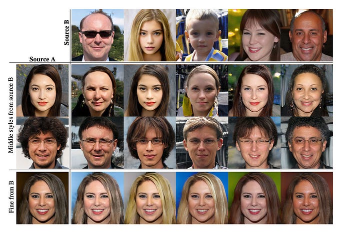
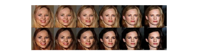
As shown below, we use the latent factors that generate image “source B” to derive the coarse spatial resolutions (4×4 to 8×8) style and use that of “source A” for finer spatial resolutions. Therefore, the generated image will have high-level style such as pose, general hairstyle, face shape, and eyeglasses from source B, while all colors (eyes, hair, lighting) and finer facial features resemble A.
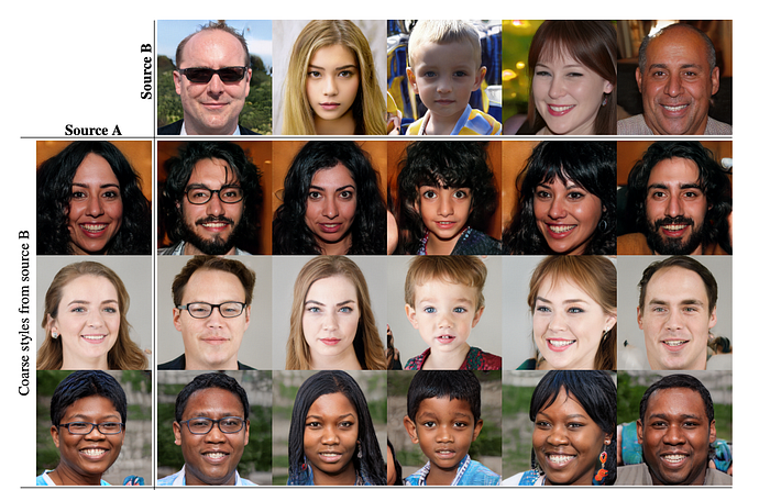
If it uses the styles of middle resolutions (16×16 to 32×32) from source B, it inherits smaller scale facial features, hairstyle, eyes open/closed from B, while the pose, general face shape, and eyeglasses from image A are preserved. In the last column, it copies the fine styles (64×64 to 1024×1024 resolution) from source B that mainly impacts the color scheme and microstructure.
In training, a certain percentage of images are generated using two random latent codes instead of one.
Training
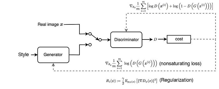
FFHQ (a dataset of human faces — Flickr-Faces-HQ) is a higher quality dataset compared to the CelebA-HQ with better coverage, like age, ethnicity, image background, and accessories such as eyeglasses, hats, etc. In StyleGAN, the CelebA-HQ dataset will be trained with WGAN-GP as the loss function while FFHQ will use the non-saturated GAN loss with R₁ regularization below.
Truncation trick in W
Low probability density region in z or w may not have enough training data to learn it accurately.
So when generating images, we can avoid those regions to improve the image quality at the cost of the variation. This can be done in truncating z or w. In StyleGAN, it is done in w using:
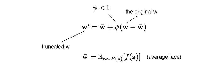
where ψ is called the style scale.
But truncation is done at the low-resolution layers only (say 4×4 to 32×32 spatial layers with ψ = 0.7). This ensures the high-resolution details are not affected.
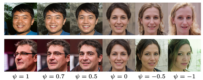
When ψ is set to 0, it generates the average face as shown below. As we adjust the value of ψ, we can see how attributes like viewpoint, glasses, age, coloring, hair length, and gender are flipped, e.g. from having an eyeglass to none.
Perceptual path length
StyleGAN paper also introduces a new metric in measuring GAN’s performance called perceptual path length. In GAN, we gradually change one particular dimension in the latent factor z to visualize its semantic meaning.
Such kind of interpolation in the latent-space can yield surprisingly non-linear visual changes. For example, features that are absent in both ends may appear in the middle. This is a sign that the latent space, as well as the factors of variation, is highly entangled. Therefore, we can quantify these changes by measuring the accumulated changes as the interpolation is performed. First, we can use the VGG16 embedding to measure the perceptual difference between two images. If we subdivide a latent space interpolation path into linear segments, we can add all the perceptual differences over each segment together. The lower the value, the better the GAN image should be. For simplicity here, please refer to the StyleGAN paper for the exact mathematical definition.
StyleGAN Issues
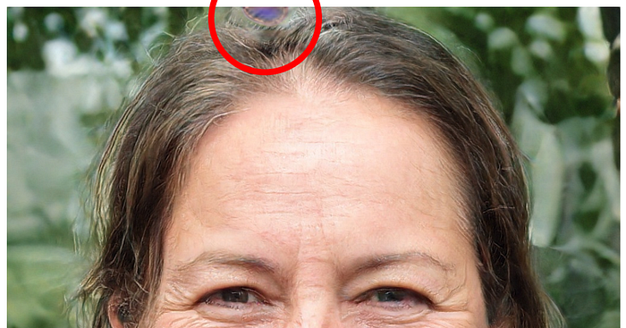
Blob-like artifacts (resembling water droplets) are observed in StyleGAN generated images which are more obvious at examining the intermediate feature maps inside the generator network. This issue seems to occur at 64×64 resolution in all feature maps and get worse in higher resolution.
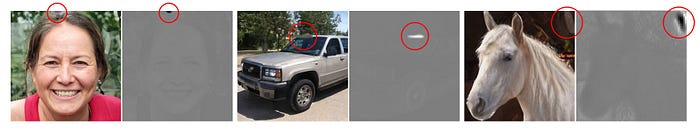
GAN technology has been improved so well that I find it easier to zoom into the pictures and look for areas where the image pattern looks abnormal in detecting fake images.
In the StyleGAN2 paper, it traces the problem to the instance normalization used in AdaIN. AdaIN is originally targeted for style transfer to replace the style of one image with another which in the process some important information of the input feed will be lost.
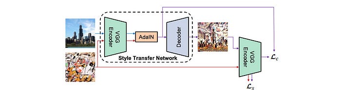
As quoted from the StyleGAN2 paper:
We pinpoint the problem to the AdaIN operation that normalizes the mean and variance of each feature map separately, thereby potentially destroying any information found in the magnitudes of the features relative to each other. We hypothesize that the droplet artifact is a result of the generator intentionally sneaking signal strength information past instance normalization: by creating a strong, localized spike that dominates the statistics, the generator can effectively scale the signal as it likes elsewhere
In addition, StyleGAN2 proposes an alternative design in solving issues that occurred in using progressive growing which its purpose is to stabilize high-resolution training.
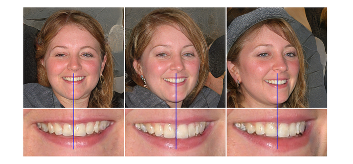
As shown above, the center locations of the teeth (blue line) do not change even the generated faces are turning to the right when progressive growing is used.
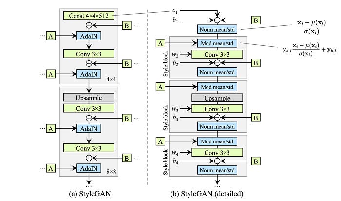
Before discussing StyleGAN2, let’s redraw the StyleGAN design as the one on the right. The design is the same in which the AdaIN module is split into two modules. Bias is added which is omitted in the original diagram. (Note, no design change is made so far.)
StyleGAN2
Weight demodulation
With supports from the experimental results, the changes in StyleGAN2 made include:
- Remove (simplify) how the constant is processed at the beginning.
- The mean is not needed in normalizing the features.
- Move the noise module outside the style module.
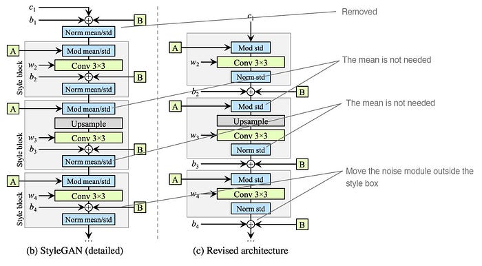
Next, StyleGAN2 simplifies the design as below with weight demodulation. It revisits the instant normalization design (Norm std) with the purpose of replacing it with another normalization method that does not have the blob-like artifacts. The right diagram below is the new design with weight demodulation.
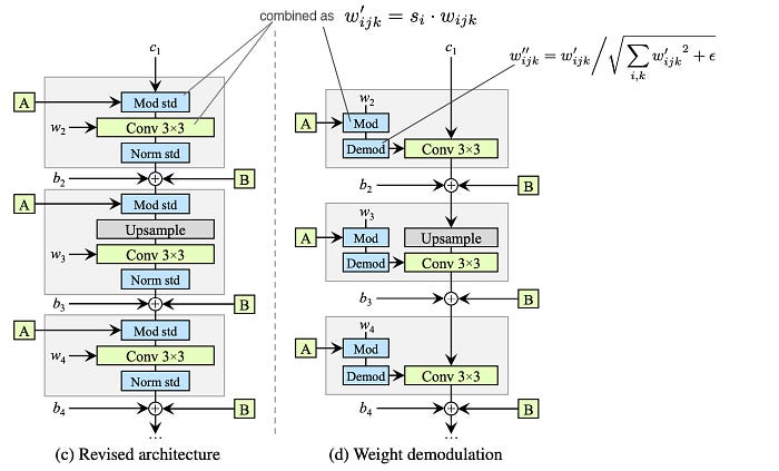
Weight demodulation adds the following changes:
- The modulation (mod std) followed by the convolution (Conv 3×3) can be combined as scaling the convolution weights and implement as Mod above. (This does not change the model design.)

where i is the input feature map i.
2. Then it normalizes the weight with (Demod)

The new weight is normalized as

with a small ε added to avoid numerical instability. Even though it is not mathematically the same as the instant normalization, it normalizes the output feature map to have a standard unit standard deviation and achieve similar goals as other normalization methods (in particular, making the training more stable). Experiment results show that the blob-like artifacts are resolved.
StyleGAN2 improvement
Again, we will discuss the improvement one at a time. The diagram below summarizes the changes and the FID score improvement (the smaller the better).
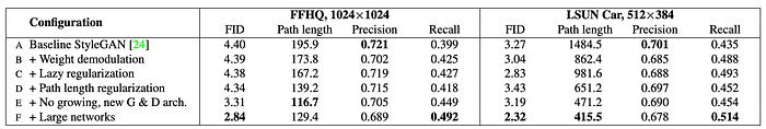
Lazy regularization
StyleGAN applies R₁ regularization with the FFHQ dataset. It turns out that it is no harm to ignore the regularization cost most of the time during the cost calculation. Indeed, even adding regularization cost only once every 16 mini-batches, the model performance remains the same while it reduces the computation cost.
Path length regularization
As discussed before, path length can be used to measure GAN’s performance. Another possible sign of trouble is the path distance varies a lot between different segments along the interpolation path. In short, we prefer the linear interpolated points to have similar image distances between consecutive points. In another word, the same displacement in the latent space should yield the same magnitude change in the image space, regardless of the value of the latent factor. Therefore, we add a regularization below
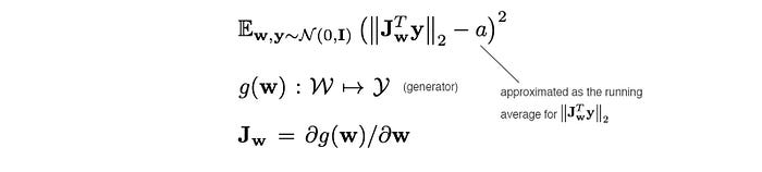
Cost is added when the change in the image space is different from the ideal expected displacement. The change in the image space is computed from the gradient which is available for the backpropagation and the expected displacement is approximated by the running average so far. We will not go into the details here. If you want to know the exact detail, the best way is to run the debugger for the code.
Progressive growth
StyleGAN uses the progressive growth idea to stabilize the training for high-resolution images. With the progressive growth issue mentioned before, StyleGAN2 searches for alternative designs that allow network design with great depth and good training stability. For ResNet, this is done with skip connection. So StyleGAN2 explores the skip connection design and other residual concepts similar to ResNet. For these designs, we use bilinear filtering to up/downsampling the previous layers and try to learn the residual values of the next layer instead.
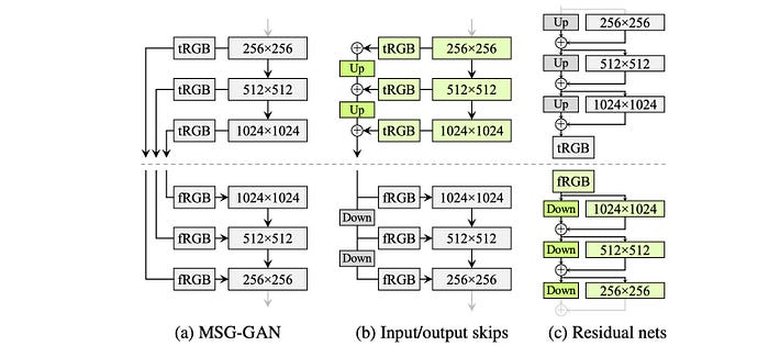
Here is the MSG-GAN design with the skip connection between the discriminator and the generator.

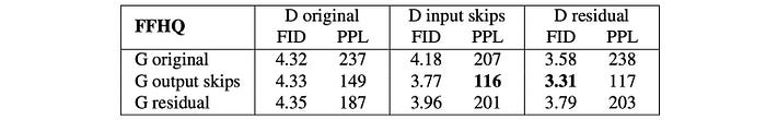
Here is the performance improvement using different approaches.
Large networks
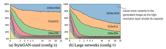
After all these changes, further analysis is done to see how the fine resolution layers are impacting the image generation. The paper measures the variant of the images that contributed from different model layers. The left diagram below plots the contribution of each layer with the horizontal axis being the training progress. In the beginning, the lower resolution layers should dominate. Nevertheless, as more training iterations are done, the contribution from the high-resolutions layer should dominate. Nevertheless, the contributions from the high-resolution layers in specific the 1024 × 1024 layers are not contributed as much as it should be. It was suspected that the capacity of these layers is not large enough. Indeed, when the number of feature maps is double in the high-resolution layers, it shows its impact significantly improved (the right diagram).
Credits & References
A Style-Based Generator Architecture for Generative Adversarial Networks
Analyzing and Improving the Image Quality of StyleGAN
Implementations
