GAN — Wasserstein GAN & WGAN-GP

11 min readJun 14, 2018

Training GAN is hard. Models may never converge and mode collapses are common. To move forward, we can make incremental improvements or embrace a new path for a new cost function. Do cost functions matter in the GAN training? This article is part of the GAN series which looks into the Wasserstein GAN (WGAN) and the WGAN-Gradient penalty in details. The equations for Wasserstein GAN look very unapproachable. In reality, they are pretty simple and we will explain them with examples.

Earth-Mover (EM) distance/ Wasserstein Metric

Let’s complete a simple exercise on moving boxes. We get 6 boxes and we want to move them from the left to the locations marked by the dotted square on the right. For box #1, we move it from location 1 to location 7. The moving cost equals to its weight times the distance. For simplicity, we will set the weight to be 1. Therefore the cost to move box #1 equals to 6 (7–1).

The figure below presents two different moving plans γ. The tables in the right illustrates how boxes are moved. For example, in the first plan, we move 2 boxes from location 1 to location 10 and the entry γ(1, 10) is therefore set to two. The total transport cost of either plan below is 42.

However, not all transport plans bear the same cost. The Wasserstein distance (or the EM distance) is the cost of the cheapest transport plan. In the example below, both plans have different cost and the Wasserstein distance (minimum cost) is two.

Let’s throw in some complicated terms before explaining it. The Wasserstein distance is the minimum cost of transporting mass in converting the data distribution q to the data distribution p. The Wasserstein distance for the real data distribution Pr and the generated data distribution Pg is mathematically defined as the greatest lower bound (infimum) for any transport plan (i.e. the cost for the cheapest plan):

From the WGAN paper:

Π(Pr, Pg) denotes the set of all joint distributions γ(x, y) whose marginals are respectively Pr and Pg.

Don’t get scared by the mathematical formula. The equation above is the equivalent of our example in the continuous space. Π contains all the possible transport plan γ.

We combine variable x and y to form a joint distribution γ(x, y) and γ(1, 10) is simply how many boxes at location 10 is from location 1. The number of boxes in location 10 must originally come from any position, i.e. ∑ γ(*, 10) = 2. That is the same as saying γ(x, y) must have marginals Pr and Pg respectively.

KL-Divergence and JS-Divergence

Before advocating any new cost functions, let’s look at the two common divergences used in generative models first, namely the KL-Divergence and the JS-Divergence.

where p is the real data distribution and q is the one estimated from the model. Let’s assume they are Gaussian distributed. In the diagram below, we plot p and a few q having different means.

Below, we plot the corresponding KL-divergence and JS-divergence between p and q with means ranging from 0 to 35. As anticipated, when both p and q are the same, the divergence is 0. As the mean of q increases, the divergence increases. The gradient of the divergency will eventually diminish. We have close to a zero gradient, i.e. the generator learns nothing from the gradient descent.

Criticizing is easy. In practice, GAN can optimize the discriminator easier than the generator. Minimizing the GAN objective function with an optimal discriminator is equivalent to minimizing the JS-divergence (proof). As illustrated above, if the generated image has distribution q far away from the ground truth p, the generator barely learns anything.

Arjovsky et al 2017 wrote a paper to illustrate the GAN problem mathematically with the following conclusions:

An optimal discriminator produces good information for the generator to improve. But if the generator is not doing a good job yet, the gradient for the generator diminishes and the generator learns nothing (the same conclusion we just explain).

The original GAN paper proposes an alternative cost function to address this gradient vanishing problem. However, Arjovsky illustrates the new functions have large variance of gradients that make the model unstable.

Arjovsky proposes adding noise to generated images to stabilize the model.

For more details, here is another article in our series that summarizes some of the important mathematical claims.

Wasserstein Distance

Instead of adding noise, Wasserstein GAN (WGAN) proposes a new cost function using Wasserstein distance that has a smoother gradient everywhere. WGAN learns no matter the generator is performing or not. The diagram below repeats a similar plot on the value of D(X) for both GAN and WGAN. For GAN (the red line), it fills with areas with diminishing or exploding gradients. For WGAN (the blue line), the gradient is smoother everywhere and learns better even the generator is not producing good images.

Wasserstein GAN

However, the equation for the Wasserstein distance is highly intractable. Using the Kantorovich-Rubinstein duality, we can simplify the calculation to

where sup is the least upper bound and f is a 1-Lipschitz function following this constraint (see here for more info on the Lipschitz constraint):

So to calculate the Wasserstein distance, we just need to find a 1-Lipschitz function. Like other deep learning problem, we can build a deep network to learn it. Indeed, this network is very similar to the discriminator D, just without the sigmoid function and outputs a scalar score rather than a probability. This score can be interpreted as how real the input images are. In reinforcement learning, we call it the value function which measures how good a state (the input) is. We rename the discriminator to critic to reflect its new role. Let’s show GAN and WGAN side-by-side.

GAN:

WGAN

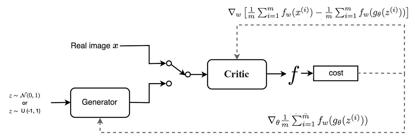
The network design is almost the same except the critic does not have an output sigmoid function. The major difference is only on the cost function:

However, there is one major thing missing. f has to be a 1-Lipschitz function. To enforce the constraint, WGAN applies a very simple clipping to restrict the maximum weight value in f, i.e. the weights of the discriminator must be within a certain range controlled by the hyperparameters c.

Algorithm

Now we can put everything together in the pseudo-code below.

Experiment

Correlation between loss metric and image quality

In GAN, the loss measures how well it fools the discriminator rather than a measure of the image quality. As shown below, the generator loss in GAN does not drop even the image quality improves. Hence, we cannot tell the progress from its value. We need to save the testing images and evaluate it visually. On the contrary, WGAN loss function reflects the image quality which is more desirable.

Improve training stability

Two significant contributions for WGAN are

it has no sign of mode collapse in experiments, and
the generator can still learn when the critic perform well.

As shown below, even though we remove the batch normalization in DCGAN, WGAN can still perform.

WGAN — Issues

Lipschitz constraint

Clipping allows us to enforce the Lipschitz constraint on the critic’s model to calculate the Wasserstein distance.

Quote from the research paper: Weight clipping is a clearly terrible way to enforce a Lipschitz constraint. If the clipping parameter is large, then it can take a long time for any weights to reach their limit, thereby making it harder to train the critic till optimality. If the clipping is small, this can easily lead to vanishing gradients when the number of layers is big, or batch normalization is not used (such as in RNNs) … and we stuck with weight clipping due to its simplicity and already good performance.

The difficulty in WGAN is to enforce the Lipschitz constraint. Clipping is simple but it introduces some problems. The model may still produce poor quality images and does not converge, in particular when the hyperparameter c is not tuned correctly.

The model performance is very sensitive to this hyperparameter. In the diagram below, when batch normalization is off, the discriminator moves from diminishing gradients to exploding gradients when c increases from 0.01 to 0.1.

Model capacity

The weight clipping behaves as a weight regulation. It reduces the capacity of the model f and limits the capability to model complex functions. In the experiment below, the first row is the contour plot of the value function estimated by WGAN. The second row is estimated by a variant of WGAN called WGAN-GP. The reduced capacity of WGAN fails to create a complex boundary to surround the modes (orange dots) of the model while the improved WGAN-GP can.

Wasserstein GAN with gradient penalty (WGAN-GP)

WGAN-GP uses gradient penalty instead of the weight clipping to enforce the Lipschitz constraint.

Gradient penalty

A differentiable function f is 1-Lipschitz if and only if it has gradients with norm at most 1 everywhere.

In specific, Appendix A in WGAN-GP paper proves that

Points interpolated between the real and generated data should have a gradient norm of 1 for f.

So instead of applying clipping, WGAN-GP penalizes the model if the gradient norm moves away from its target norm value 1.

λ is set to 10. The point x used to calculate the gradient norm is any points sampled between the Pg and Pr. (It will be easier to understand this with the pseudo-code later.)

Batch normalization is avoided for the critic (discriminator). Batch normalization creates correlations between samples in the same batch. It impacts the effectiveness of the gradient penalty which is confirmed by experiments.

By design or not, some new cost functions add gradient penalty to the cost function. Some is purely based on empirical observation that models misbehave when the gradient increases. However, gradient penalty adds computational complexity that may not be desirable but it does produce some higher-quality images.

Algorithm

Let’s look into the pseudo code in detailing how the sample point is created and how the gradient penalty is computed.

WGAN-GP Experiments

WGAN-GP enhances training stability. As shown below, when the model design is less optimal, WGAN-GP can still create good results while the original GAN cost function fails.

Below is the inception score using different methods. The experiment from the WGAN-GP paper demonstrates better image quality and convergence comparing with WGAN. However, DCGAN demonstrates slightly better image quality and it converges faster. But the inception score for WGAN-GP is more stable when it starts converging.

So what is the benefit of WGAN-GP if it cannot beat DCGAN? The major advantage of WGAN-GP is its convergency. It makes training more stable and therefore easier to train. As WGAN-GP helps models to converge better, we can use a more complex model like a deep ResNet for the generator and the discriminator. The following are the inception score (the higher the better) using ResNet with WGAN-GP.