Machine Learning —Expectation-Maximization Algorithm (EM)

Chicken and egg problems are major headaches for many entrepreneurs. Many machine learning (ML) problems deal with a similar dilemma. If we know A, we can determine B. Or, if we know B, we can determine A. Either way solves the ML problem. Unfortunately, we don’t know A or B. But in ML, it can be solved by one powerful algorithm called Expectation-Maximization Algorithm (EM).
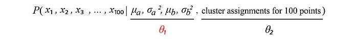
Let’s illustrate it easily with a clustering example, called Gaussian Mixture Model (GMM). GMM finds an optimal way to group 100 data points (x₁, x₂, …, x₁₀₀) into two clusters. A Gaussian distribution (with parameter μ, σ²) will be used to model its likelihood, i.e. the probability that a data point xᵢ belongs to a specific cluster is:

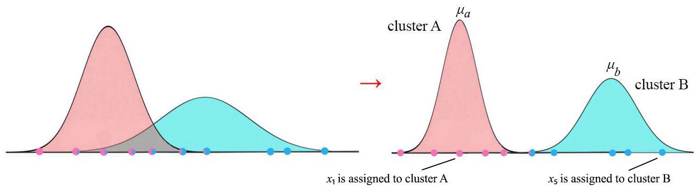
Why do we call it the chicken and egg problem? If we know the mean and the variance of both clusters, we know where these points belong to. If we know where they belong, we can calculate the Gaussian parameters for both clusters. But we know neither one.
But let’s take a broader view of the problem. Let’s assume z are the latent variables for x. If we know how to model and solve p(x|z), z can be found by MLE using the following objective:

And you don’t need the EM algorithm. If this is not the case, we can optimize the log-likelihood of the observation x. By summing over all possibilities of z, we can take its derivative to find the optimal z.

However, as shown before, the gradient involving the log of a sum can be intractable.
As a side note, there is another serious problem. In many ML problems, we model p(x|z) as an exponential family of distribution which has a concave log-likelihoods. But now, p(x) is a weighted sum of p(x|z). The sum is no longer concave or convex. So it is not easy to find the global optimum.

Many ML problems are much easier to model and to be solved by introducing another latent variable θ₂. Assuming that if we have x and θ₁ (a.k.a. z) fixed, we can model the distribution of θ₂ as:

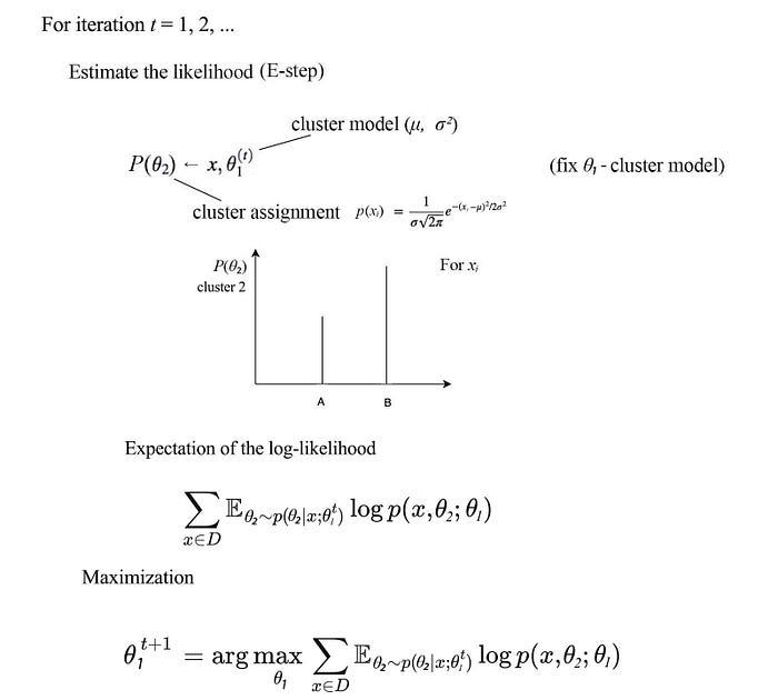
To find θ₁, we can simply find the optimal θ₁ in maximizing the expected log-likelihood above. Intuitively, we find the optimal θ₁ for the log-likelihood of the evidence given the distribution of θ₂ calculated by θ₁.

This equation is in the form of the sum of the log. It is concave. It is not hard to optimize. This turns into our easy chicken and egg problem.

Many ML problems can be solved in alternating steps with one latent variable fixed at a time. First, we start with an initial guess. We continue our expectation formularization and maximization iteratively, the solution will converge. That is why we call the method Expectation-Maximization.
Gaussian Mixture Model GMM
Let’s detail the solution more with the GMM. In our problem, we are interested in learning the Gaussian parameters θ₁ for the two clusters.
And in inference, we are interested in predicting the cluster assignment of the new data point. In this prediction, we need θ₁ only. So how do we find the optimal θ₁ from the training data?

We start with a random guess for the clustering model θ₁ (μa, σa², μb, σb²). To solve the problem, we introduce the cluster assignments P(θ₂) for each sample data point. And compute the chance that xᵢ belongs to a specific cluster with:

For example, the data point xᵢ=3 may have a 0.2 chance to be in cluster A and 0.8 chance to be in cluster B. Then based on this distribution P(θ₂), we optimize the expected log-likelihood of the observation x w.r.t the cluster assignment (θ₁). However, θ₂ depends on θ₁ and vice versa. We are working with multiple moving parts in a circular loop.
So, we fix θ₁ and derive θ₂. Then we optimize θ₁ with θ₂ fixed. We repeat the iterations until θ₁ converge. In each iteration, our objective will improve. Assuming a limited precision, we are dealing with a finite space for θ₁ and θ₂. Therefore, there is a finite step for θ₁ and θ₂ to improve and our iteration would at least reach a local optimal.
In the EM-algorithm, the E-step fix the Gaussian models θ₁ (μa, σa², μb, σb²) and compute the assignment probabilities P(θ₂). In the EM algorithm, we assume we know how to model p(θ₂ |x, θ₁) easily. If not, the EM algorithm will not be helpful. In the E-step, we apply a Gaussian model where θ₂ ∈ {a, b} and we compute p(aᵢ) and p(bᵢ) for each data point i.
In the M-step, we maximize p(x | θ₁) w.r.t. θ₁. This is done by marginalized over θ₂. It turns out this can be done pretty straight forward in GMM. For simplicity, we write p(aᵢ) as aᵢ below. Here are the equations used for GMM. (More details can be found here.)

Mathematical model
(Credit: the equations in this section are originated from here.)
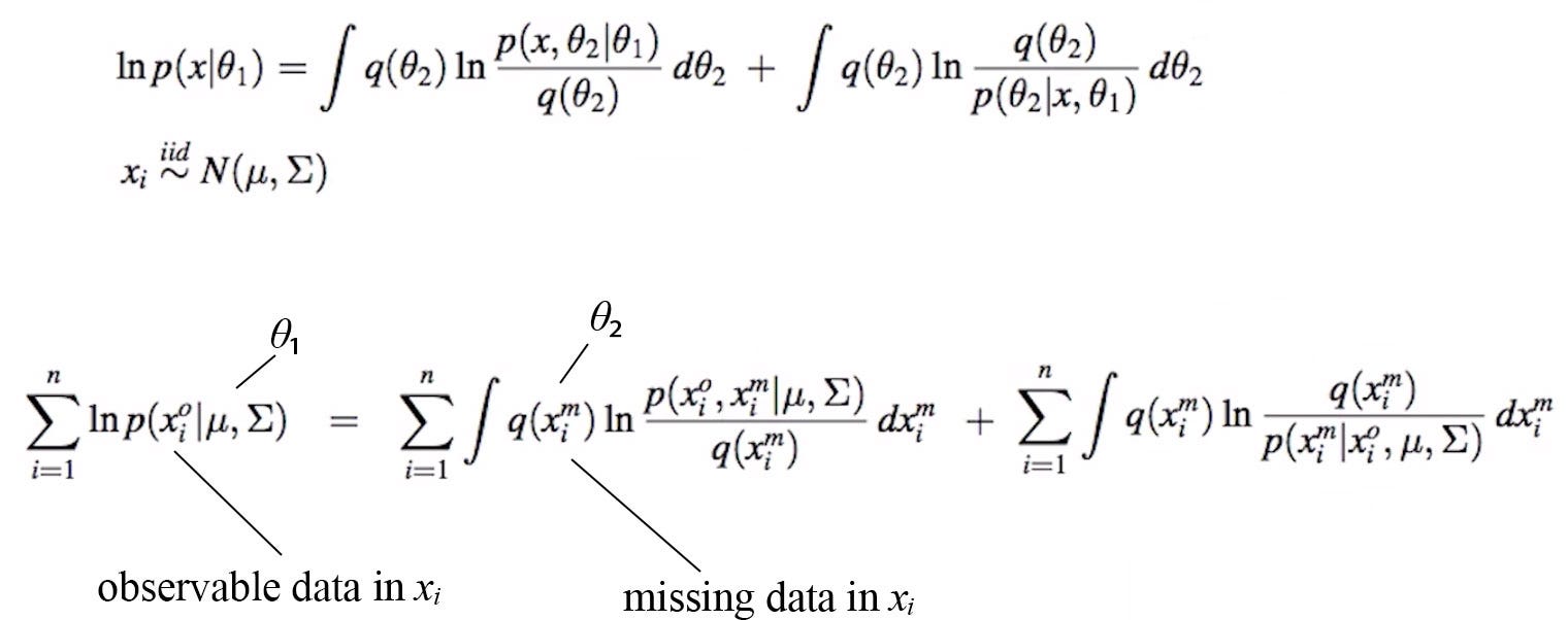
Our GMM example is a special case for the EM algorithm. In this section, we will discuss the Math in greater details and generalize the concept a little bit more. Given xᵢ is i.i.d., data can be drawn from the same distribution Ɲ and independent of each other.

Therefore, maximizing the likelihood of the observation is equivalent to maximizing the sum of log-likelihood of each observation.

Expectation-maximization (EM) algorithm is a general class of algorithm that composed of two sets of parameters θ₁, and θ₂. θ₂ are some un-observed variables, hidden latent factors or missing data. Often, we don’t really care about θ₂ during inference. But if we try to solve the problem, we may find it much easier to break it into two steps and introduce θ₂ as a latent variable. First, we derive θ₂ from the observation and θ₁. Then we optimize θ₁ with θ₂ fixed. We continue the iterations until the solution converges.
In the M-step, we maximize the log-likelihood of the observations w.r.t. θ₁. The log-likelihood ln p(x|θ₁) can be decomposed as the following with the second term being the KL-divergence (proof).
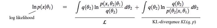
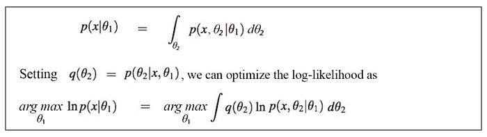
where q(θ₂) can be any distribution.
Now, let’s make the R.H.S. as simple as possible so we can optimize it easily. First, let’s pick a choice for q(θ₂). A natural one will be p(θ₂|x, θ₁) — the probability of θ₂ given the observation and our model θ₁. By setting q(θ₂) = p(θ₂|x, θ₁), we get a nice bonus. The KL-divergence term becomes zero. Now our log-likelihood can be simplified to
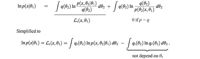
Since the second term does not change w.r.t. θ₁, we can optimize the R.H.S. term below.
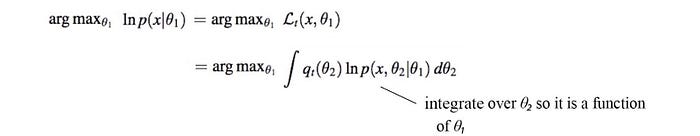
This is the expected log-likelihood over θ₂.
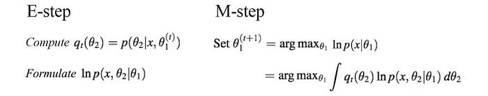
Let’s recap. In the E-step (expectation estimation step), we compute q(θ₂) and re-establish the equation for the log-likelihood ln p(x |θ₁).

In the M-step (maximization step), we optimize this expected log-likelihood w.r.t. θ₁.

Here is the EM-algorithm:
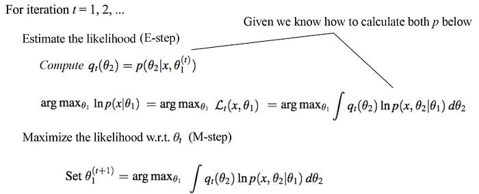
For the solution to work, we assume we know how to model p(θ₂ | x, θ₁) and p(x, θ₂ | θ₁). The success of the EM algorithm subjects to how simple are they and how easy to optimize the later one. In GMM, this can be done easily.
Narrative of the EM algorithm
Let’s summarize what we learn.
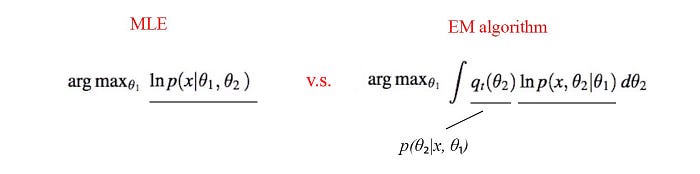
In some ML problems, it is intractable to solve the problem with our perceived model parameter θ₁. Instead, we solve the problems in alternating steps by adding latent parameters θ₂. By breaking down the problem, the equations involve θ₁ → θ₂ → θ₁. And this problem can be solved much simpler. Our objective is solving either the L.H.S. or the R.H.S. below.

If we can model and optimize p(x | θ₁, θ₂) easily, we don’t need the EM algorithm. Just use MLE. But as shown below, it is not the case for GMM. The log of the sum is intractable but the sum of the log is tractable.
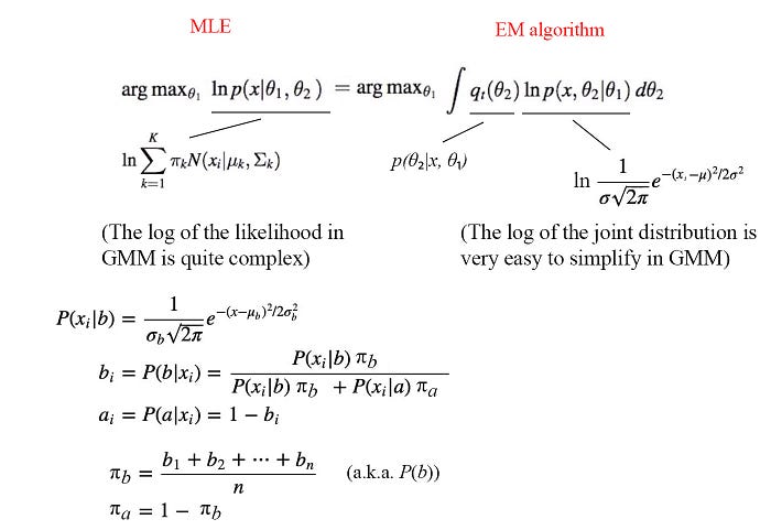
For the GMM problem, the joint distribution p(x, θ₂ | θ₁) in the EM algorithm is modeled as a Gaussian. Its log is simple. q(θ₂) is set to p(θ₂ | x, θ₁) with θ₁ fixed. Optimizing this formularization is easy. On the contrary, the equations for p(x | θ₁, θ₂) is very complex. Therefore, we choose the EM algorithm to solve GMM.
So if the problem can be modeled easier with its subcomponents (the joint distribution) and we know how to model p(θ₂ | x, θ₁) easily, EM algorithm will have an edge over MLE (otherwise, no). Another example in demonstrating this idea with the PCA can be found here.
In MLE or EM, θ₁ and θ₂ may depend on each other. Therefore, we optimize θ₁ or θ₂ one at a time with the other fixed. Iterating between alternating steps, the solution will converge.
Minorize-Maximization MM algorithm
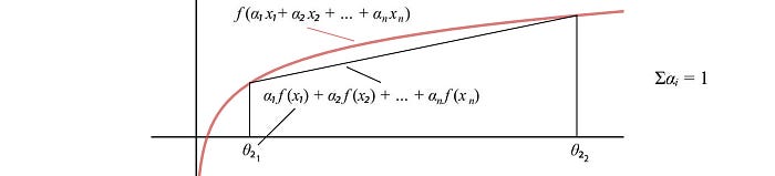
The EM algorithm can be treated as a special case for the MM algorithm. With Jensen’s inequality, we can establish a lower bound for the log-likelihood as below for any distribution q.
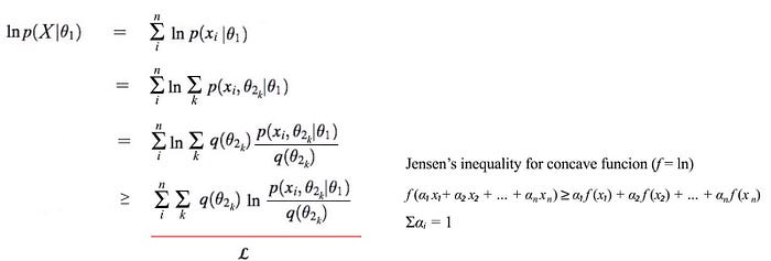
In the diagram below, we demonstrate Jensen’s inequality for the log function with k = 2 and q(θ₂_k) as αᵢ below.
Without too much elaboration, let’s understand the MM algorithm graphically. As mentioned before, the log-likelihood loss function L can be in some shape that is hard to optimize. We will use the MM method to optimize it instead.
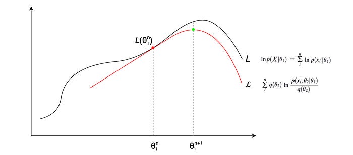
𝓛 is the lower bound for the log-likelihood loss function L that we want to optimize. At iteration n, we compute q(θ₂) = p(θ₂ | x, θ₁ⁿ). 𝓛 will be the same as L at θ₁ⁿ (the lower bound is tight). At the same time, 𝓛 with this q(θ₂) establishes a lower bound for L. 𝓛 is in the form of the sum of the log and it is easier to optimize. Therefore, we optimize 𝓛 to find a new optimal for θ₁ (the green dot). Then, we can use the new optimal θ₁ to compute q(θ₂) and establish a new lower bound 𝓛.
As shown below, as we keep iterating, we can at least reach a local optimal for L. Intuitively, for a random guess on θ, we establish a lower bound function 𝓛. We find the optimal point for 𝓛 and use it as the next guess. We continue finding a lower bound function and optimize it as a way to optimize a function f. The MM algorithm takes advantage of the idea that f may be very hard to optimize but we can find lower bound functions that are much easier.
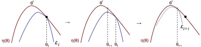
A detail mathematical proof that each iteration improves the likelihood can be found here.
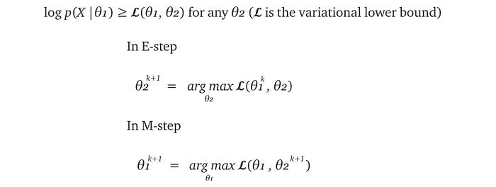
The EM algorithm becomes
Missing data
Previously, we introduce latent variable θ₂ to complement θ₁ to solve our optimization problem. The EM algorithm can be used to estimate missing data in the training dataset also. For example, the training data may be collected from user surveys. But users may answer a subset of questions only and there will be different missing data in each survey. In this situation, θ₂ will be the missing data that we want to model and θ₁ is the answers provided in the surveys. Another example is removing noise in an image which we consider the noise as the missing data. Here is how we formulate the log-likelihood using our EM equations.
We will not elaborate on the solution further but the steps to find the solution can be found here.
Terms
Here is the recap of some terminology.

Variational inference (optional)
At one point, we should suspect variational inference and EM-algorithm are closely related as they both work with the log-likelihood and minimize the KL-divergence.
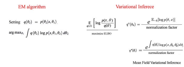
In the variational inference, we approximate the posterior p(x, z ; θ )with a tractable distribution q. We maximize the evidence lower bound ELBO below to find the optimal q*:

ELBO fulfills:

i.e. We maximize the log-likelihood if q equals p(z|x; θ).
Therefore, the EM algorithm can be viewed as optimizing the ELBO over θ₂ at the E-step and over θ₁ at the M-step. By setting q to p(z|x; θ), we maximize the ELBO.
Previously, we calculate p(θ₂|x; θ₁) explicitly ourself. In variational inference, we approximate it with tractable distributions. In fact, EM can adapt the same strategy in the E-step to approximate p(θ₂|x; θ₁) with tractable distributions. Of course, the complexity will be significantly increased.
