Machine Learning — Graphical Model

22 min readJun 19, 2019

One major difference between Machine Learning (ML) and Deep Learning (DL) is the amount of domain knowledge sought to solve a problem. ML algorithms regularly exploit domain knowledge. However, the solution can be biased if the knowledge is incomplete. However, if it is done correctly, we can solve problems more efficiently.

The Graphical model (GM) is a branch of ML which uses a graph to represent a domain problem. Many ML & DL algorithms, including Naive Bayes’ algorithm, the Hidden Markov Model, Restricted Boltzmann machine and Neural Networks, belong to the GM. Studying it allows us a bird’s eye view on many ML algorithms. In this article, we focus on the basic in representing a problem using a graphical model. Later in this series, we will discuss how inference is made and how the model is trained.

Probabilistic graphical modeling combines both probability and graph theory. The probabilistic part reason under uncertainty. So we can use probability theory to model and argue the real-world problems better. The graph part models the dependency or correlation.

In GM, we model a domain problem with a collection of random variables (X₁, . . . , Xn) as a joint distribution p(X₁, . . . , Xn). The model is represented by a graph. Each node in the graph represents a variable with each edge representing the dependency or correlation between two variables.

For example, the sprinkler problem above is modeled by three variables:

whether the sprinkler is automatically on or off,
whether it is raining, and
whether the grass is wet.

And we model the problem with the joint probability

The power of the joint probability may not be obvious now. But it answers a wide spectrum of queries (inference) including

The likelihood of the observations P(E) — the chance of the lab results (Evidence E).
The marginal probability P(X₁), P(X₁, X₃), etc … — the chance of having Alzheimer when you are 70.
Conditional probability (or a posterior belief based on evidence), P(Y|E) — the chance of having Alzheimer given your parent has it.
Maximum a Posterior (MAP), arg max P(X, E) — the most likely disease given the lab results.

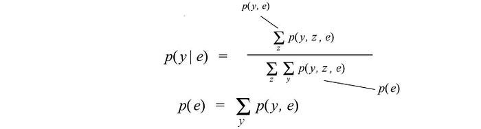
For example, the marginal probability of having the grass wet is computed by summing over other variables. For the conditional probability, we can first apply Bayes’ Theorem followed by the corresponding marginal probabilities.

Recap

In GM, we choose a graph to represent information and their relationship in a dense form. We make inferences in the form of marginal probability P(x₁), P(x₁, x₂), conditional probability P(x | e), or MAP arg max P(x, e). And we build a model by maximizing the likelihood of our collected sample. In conjunction with Bayes’ theorem, it forms the basic framework in capturing uncertainty in the real-word with probability theory. Before giving an example of GM, let’s see how we model a joint distribution first.

Joint probability

Which probability distributions below is more complex? Let’s give some serious thoughts here because it helps us to understand machine learning (ML) better.

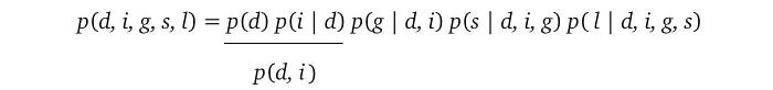
For the L.H.S. distribution, we can expand it using the chain rule.

Let’s assume that after further analysis of the domain problem, we discover the independence claims below. For example, the first claim is variable i is independent of d.

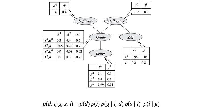
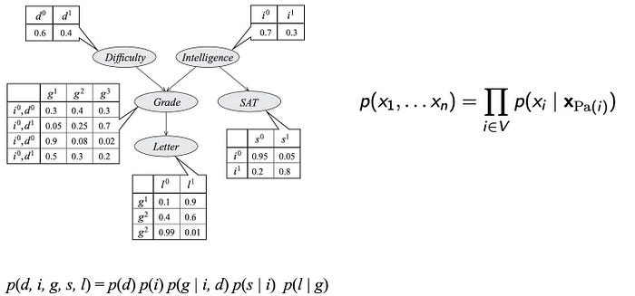
Therefore, we can simplify the R.H.S. expression as:

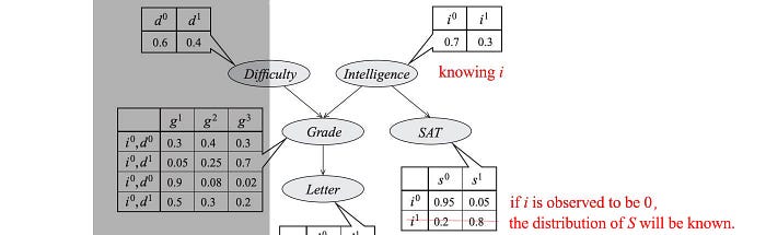
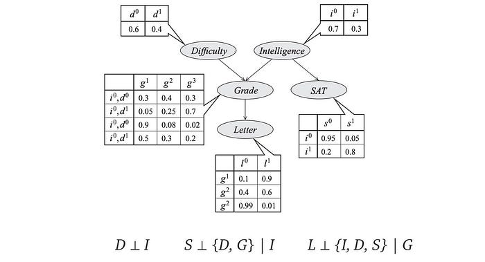
We can draw this dependency using a directed Graphical model. Each node represents a variable and to quantify the dependency, we associate a conditional probability for each node.

These model parameters are presented as the table entries below.

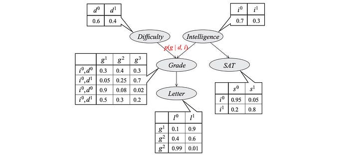
So what is the complexity for these models? p(d, i, g, s, l) have 5 variables with the possible combinations of 32 (2⁵). To model p, we sample data for 32 possibilities. On the contrary, the graph above has 4 tables with only 26 parameters.

Don’t underestimate the curse of exponential. 64 variables will have a combination of

i.e. a simple 8 × 8 grayscale image will contain enough variables (pixels) that make an ML problem too complex to solve. In ML, it is important to discover independence to break the curse of this exponential complexity, for example, Naive Bayes classifier, Hidden Markov Model, Maximum likelihood estimation with i.i.d., etc… The distribution of a variable can be calculated given all its neighbors are know. In ML, the original grand design is missing. We spot global insight through localized findings.

For many ML algorithms, the strategy is first identifying independency. Then, we model the correlations. The ability to find independence is one crtical factor in the success of a ML algorithm.

Let’s have a quick overview of the probabilistic model. This will be our foundation for further discussion.

1. Model a domain problem as a joint distribution.

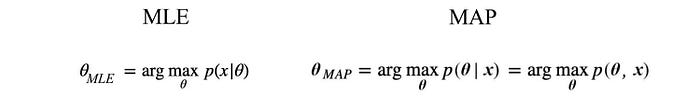
2. Learn the model parameters from the data with Maximum likelihood estimation MLE or Maximum a posteriori estimation MAP.

3. Inference. The typical inferences in ML are:

The marginal probability p(X) by summing over other variables.

Conditional probability solved with Bayes’ Theorem and marginal probabilities.

MAP inference (Maximum a posterior). For example, use Bayes’ Theorem to finding the most likely values for a set of variables given the observations.

The second inference above (the conditional probability) is simply an extension of the marginal probability. So, we will focus on the marginal inference and MAP inference for now.

In practical problems, it is hard to compute the marginal probabilities. Summing or integrating over all other variables is usually NP-hard. This is a major issue in dealing with probability models unless we can discover (or assume) enough independence, like those in the Naive Bayes Algorithm or Hidden Markov model, to reduce the complexity to polynomial.

The exact solutions for the Graphic models is usually NP-hard. The use of approximation is needed if the graphical model is too complex.

Next, we will look into details on representing a domain problem with a graph.

Bayesian network (BN)

A Bayesian network represents random variables and their dependencies using a directed acyclic graph (DAG). DAG is a directed graph with no directed cycles. Variables can be positively dependent, negatively dependent or unrelated. For example, if it rains, it has a smaller chance in turning the automatic sprinkler on. In the morning, if the grass is wet, it is because it has rained or the automatic sprinkler is on.

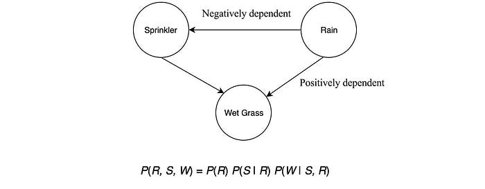
In the model above, we consider the wet grass in the morning is independent on the chance of rain or the chance of turning the automatic sprinkler on. In a Bayesian network, we join variables with a directed link in demonstrating dependency.

Let’s start with the joint probability and expand it using the chain rule.

With the Bayesian network (BN), we can simplify the conditional probability further. For example, P(S|R, W) becomes P(S|R) because S is not dependent on W. The general form of the conditional probability at each node becomes:

Now, we can simplify the data collection by just collecting the relevant data for each conditional probabilities.

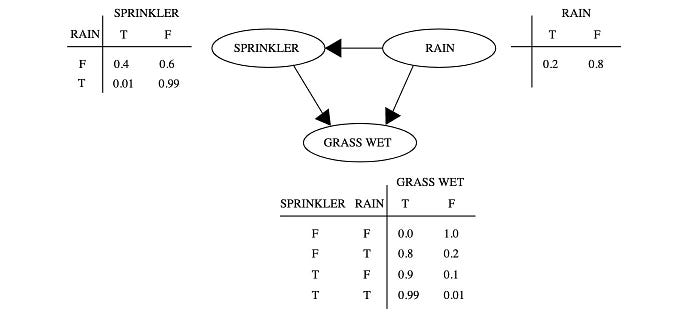
Let’s make some predictions. The conditional probability P(R|W) for rain given the grass is wet can be calculated by Bayes’ Theorem followed by the corresponding marginal probabilities.

Modified from source

The joint probability in the R.H.S. will be expanded with the conditional probabilities defined in the GM and solved with variable elimination or some approximation methods that will be discussed in later articles.

Here are another BN and the joint probability.

According to the graph, the joint probability p can be factorized as

For example, the joint distribution of this example is factorized as

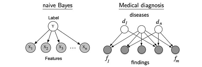
Comparing with Naive Bayes Theorem, we can use a more generic BN to model some real-life problems better. For example, given different diseases, a BN can have overlapping findings from many diseases.

Generative network

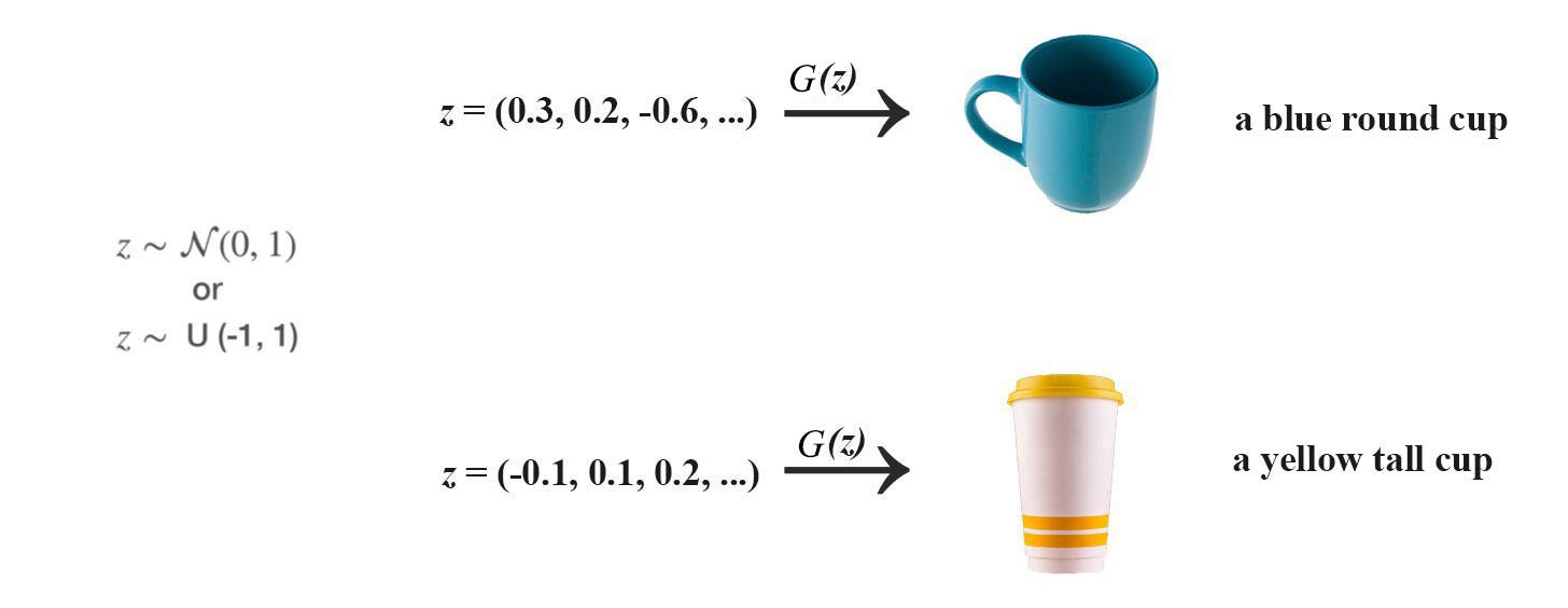
BN can be treated as a generative model — a model that can generate samples. For example, starting from the top parent nodes, we can sample and generate data according to the conditional probabilities.

This is the same principle that GAN (Generative Adversary Network) generates the raw image by first random sampling a latent variable.

Recap

A BN is a graph with each node represents a variable with one conditional probability p(x | x_parent) attached — the probability of x given its parents. We can then factorize the joint probability according to this GM.

Independence

3 + 4 equals 5 + 2. So even the formulae are different, they are identical. Given two graphs, they can model the same problem even they look different. When p is factorized according to the dependency in the Bayesian network G), we say p factorizes over G. But G is not necessarily the simplest model for our domain problem. We may miss some possible independence. However, we just make the model more complex but the solution remains sound.

Therefore, we can use the independence in determining whether two graphical models will produce the same result. Let’s conceptualize the idea of independent a little bit more.

If variables X and Y are independent (X ⊥ Y), then p(X, Y) = p(X) p(Y). First, let’s introduce the following notation in representing such independence.

If two variables A and B are independent, knowing A does not give us any information on B or vice versa.

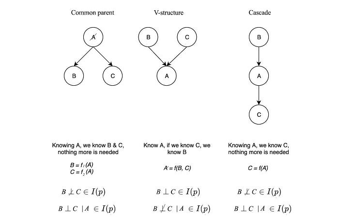
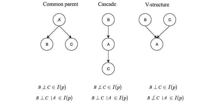
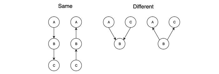
For the first diagram above, if we know A, then the probability distribution for B and C will be known and not dependent on any variable. Therefore, B & C are independent of each other given A (B ⊥ C | A ∈ I(p)).

We can prove it with the joint distribution probability derived from the graph.

But if A is unknown, knowing B can give us information on C through A. Therefore,

The graph above represents a common cause relation. We can argue such independence in an easier way without math. If the common cause is known, all its effect will be known without further information and therefore, they are not dependent on each other. If A is unknown, since all effects are linked to a common cause, therefore, all effects are related and therefore not independent.

Let’s consider the second case (v-structure).

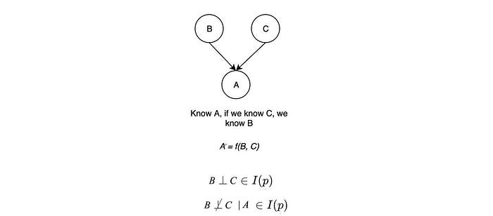
B links to C if value A is known. For example, a pedestrian is hurt (event A) if either the car or the pedestrian runs a red light. By knowing a pedestrian is hurt, we know the pedestrian is following the rule if we know the car runs a red light. Therefore B and C are not independent given A. But if A is unknown, knowing B gives us no information on C. This graph represents the common effect. If we don’t know the effect, we know nothing about the possible causes and they will be independent. But if we know the effect, B and C will be dependent.

A path in a graph is active if it carries information. In the third case below (Cascade), if we know A, then C is independent of B. We don’t need B to figure out C anymore.

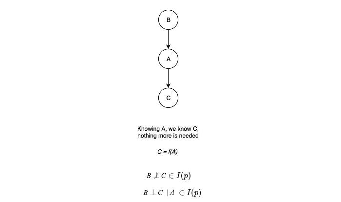
Knowing B gives us no extra information on C and therefore, the path is inactive. But if A is unknown, the path is active. B and C are d-separated (dependency separated or directional separated) if all the paths that connect them are inactive. So depending on what has been observed, we can check whether two variables are d-separated. This will be much easier in finding independence without complex math. In fact, the analysis can be done by dividing the graph into subgraphs with one of the three structures below.

For example, L is independent of {I, D, S} given G.

To evaluate whether a path is active, we can apply the following cheat sheet. In checking whether two variables are d-separated, we determine whether all possible paths between them is blocked. The cheat sheet below indicates whether a path is blocked under three different structures. So we can use that to analyze whether there is an active path between two nodes. In the cheat sheet, the shaded node represents the variable is observed.

Here is another analysis regarding variable D when C is observed. D and A are d-separated if C is observed. On the other hand, all red nodes have an active path with D if C is observed, i.e. they are not d-separated. (The graph is analyzed by this software.)

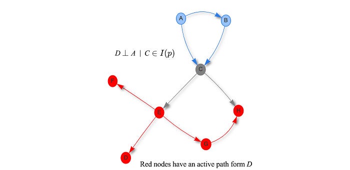
This visual analysis allows us to discover conditional dependency easily without probability theory. As shown later, it can be nasty for even simple cases. It seems that we spend an awful amount of time in studying independence. But such analysis is important. Given some known observations O, we can further prune the graph and simplify the model significantly to answer the query efficiently. For example, if C is observed in the graph above, we can drop the blue nodes for any query on the red nodes.

I-map (independence map)

Conditional independencies allow us to compare BN. Let I(G) be all conditional independencies implied by the DAG G, and I(p) be all conditional independencies hold for the joint distribution p. G is an I-map of a distribution p if I(G) ⊆ I(p). G is a minimal I-map for p if the removal of a single edge makes it not an I-map. If I(G) = I(p), G is a perfect map. Finding a perfect map may not be easy, but we want at least I(G) ⊆ I(p).

In short, if I(G) is an I-map for p, I(p) contains all the independencies of I(G), i.e. all the independencies in I(G) will not violate the rules in I(p). So the way we factorize p over G will be sound. But G is not necessarily the simplest. We may not discover all the independence. It may be more complex than it could be.

I-map is not unique. I(p) can have many I-map. For a fully connected graph G (every node is connected to each other), its independence set will be empty. Therefore, a fully connected G is always an I-map for any distribution p since I(G) = ∅ ⊆ I(p).

Without proof here, let’s make a few claims.

Finding a perfect map is not always possible in BN.
A perfect map may not be unique.
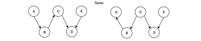
Two graphics have the same skeleton if they are the same if we ignore the arrow in the dependency.

To be perfect maps, G and G′ should have the same skeleton and the same v-structures.

Both BNs below have the same skeleton and v-structure and therefore the same.

BN examples

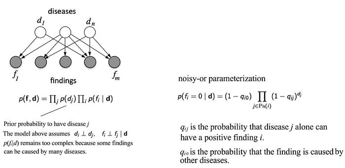
Let’s see more BN examples. We can use BN to relate diseases d and lab findings f. However, the conditional probability p(fᵢ|dⱼ) may remain too complex because many findings can be caused by many different diseases. We can simplify the joint probability further using a noisy-or parameterization below.

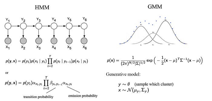
Here are the BN examples on the Hidden Markov Model and the Gaussian Mixture model.

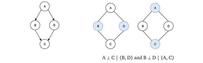
Limitations on BN

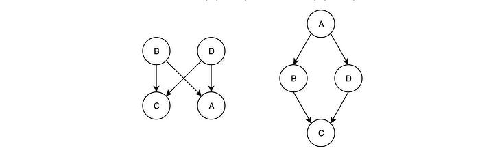
BN is a directed acyclic graph. The directed nature of the edge and the non-acyclic graph behavior make it impossible to model some independence assumptions together. Some independent assumptions cannot co-exist in a BN. For example, both BNs below can fulfill A ⊥ C | {B, D} but not B ⊥ D | {A, C}. If we want both independence together, it is not easy.

This often happens when the relationship between two variables is bi-directional. For example, friends may vote similarly. The influence is bidirectional (not directed). One solution is to introduce additional variables to the graph but that will increase the complexity of the model.

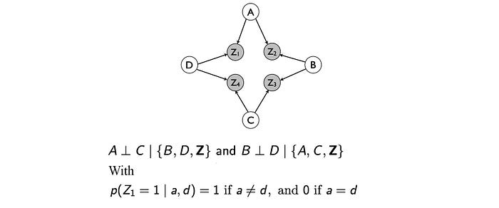
Next, we will study another type of graph that can model some independence that is not possible for BN. Nevertheless, both graphs will have different types of independence that they cannot represent. It is provided as an alternative rather than a guarantee that it works better.

Markov random fields

There are two major variants of the Graphical model. BN is one of them. The second one is the Markov random fields (MRF). MRFs models the problem with an undirected graph.

It models correlations between variables rather than dependency.

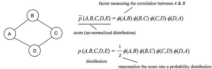
where 𝜙 is a factor function in scoring the correlations between its parameters. This replaces the conditional probability in the BN. 𝜙 can be any custom-tailored scoring function. However, p needs to be a probability distribution. Therefore, we renormalized the result by Z which is called the partition function. You will hear this term frequently in ML which behaves as a normalization factor by summing all scores for all possible combinations of the variables.

We will elaborate 𝜙 and Z further later. Here, we just introduce an abstract concept in modeling the correlations between variables. In our example above, p(A, B, C, D, E) will be high if (A, B), (B, C), (C, D) and (D, A) are highly correlated respectively. When comparing MRF with BN, we change the edge to be un-directional and use the factor functions instead of the conditional probabilities.

Let’s expand the idea further to include correlations involving more than 2 variables. A clique means a subgraph which all its nodes are interconnected. In the left diagram below, the red dots do not form a clique because the top dot is not connected to the bottom-right dot. But the rest of the diagram has cliques shown in red. A maximal clique is a clique which adding anymore node will turn it not to be a clique.

Here is a refined definition for MRF. The graph is divided into cliques. Each clique can score the correlation among its nodes. With this expanded definition, factor 𝜙 can take any non-zero number of parameters and can be different for each clique.

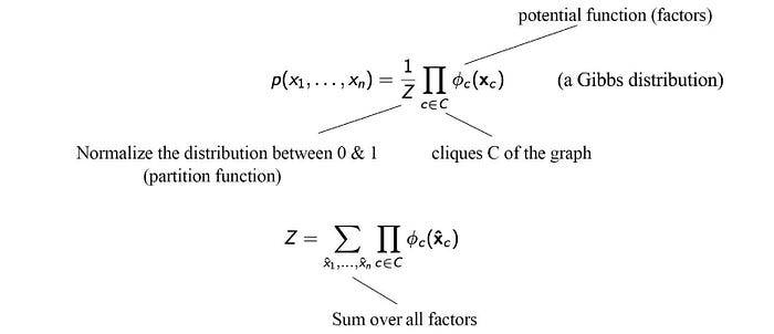
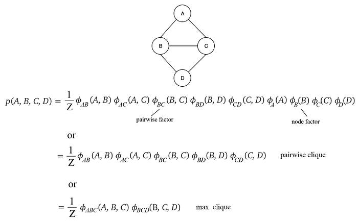
p(X) is said to be a Gibbs distribution over the MRF G if p can be factorized with the cliques in G. Our definition of MRF does not dictate which cliques to be used in the factorization, as long as they are cliques whose nodes are fully connected. Indeed, different choice of cliques results in different factorization. It is up to the decision of the model designer. All three factorizations below is valid for this MRF. The first two use pairwise clique while the last one uses the maximum clique. All can generate the same solution. The second one may require five 2-D tables and the third one requires two 3-D tables to represent the joint probability.

Here is another example:

Consider that no two neighboring houses in Cinque Terre will paint the same color. Here is the MRF model we can build for four nearby houses and the corresponding factors.

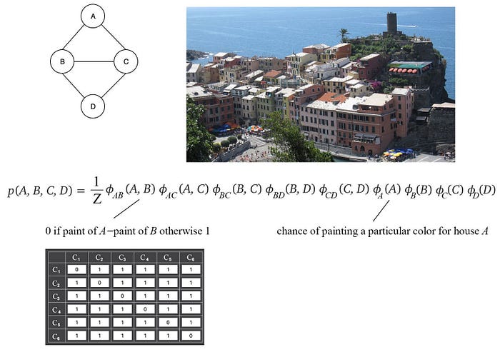
There are other choices in designing the factors 𝜙. Let’s say we have only 3 paint colors available, we can design the factors as

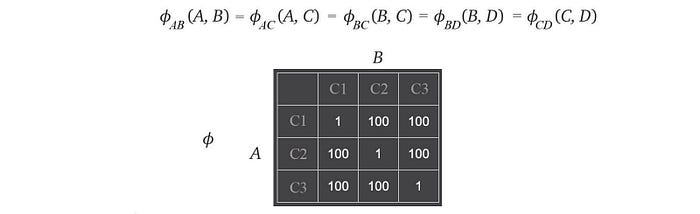
In this case, we discourage the neighboring houses to have the same color rather than completely forbidden it. We give the factor a very low score if both have the same color.

Hammersley–Clifford theorem

Without proof here, Hammersley–Clifford theorem states that if p(X)>0 for all X and G is an I-map for p(X) (the conditional independence of G is a subset of the conditional independencies of p: I(G) ⊆ I(p) ), then p(x) is a Gibbs distribution that factorizes over G.

In short, if the probability density is always positive everywhere, we can factorize p according to the cliques of G if the independence discovered by G is a subset of p.

Energy model

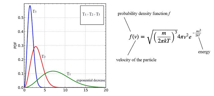
Let’s do some housekeeping work. The Graphical model has a strong root in Statistical Physics which the probability density is usually discovered as inversely proportional to the exponential of an energy function.

So GM is often explained as an energy model. Let’s introduce those terms so you may not get lost in reading some literature. Factors are also called potential functions in MRF which can be expressed in an exponential form:

θ can also be called the potential function. So just watch out for this ambiguity sometimes. So our joint probability becomes

Therefore, the probability for the configuration X is determined by the free energy H(X). In Physics, we explore different configurations X for a molecule. The non-excited state of a molecule will be the one with the lowest free energy. In some perspective, free energy is one that we are free to explore in finding the right configuration.

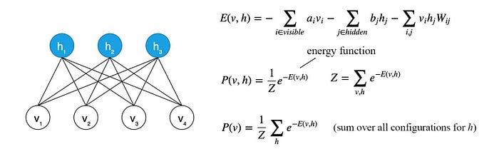
For those extra curious readers, the following is the Restricted Boltzmann Machine (RBM) and how the energy function is calculated. vᵢ and hᵢ (hidden unit/latent factor) are either 0 or 1. Wᵢⱼ accounts for the correlations between vᵢ and hⱼ. In RBM, we want to train a, b, W such that we have the lowest free energy for the training dataset.

BN is a special case of MRF which uses the conditional probability as the factor and Z=1. But similar to BN, MRF may not be the simplest model for p. But it provides an alternative that we can try to check whether it may model a problem better.

Ising model

As mentioned before, the Graphical model is heavily used in Physics. Consider a lattice of atoms. The spin of each atom is either up or down according to Quantum Mechanics.

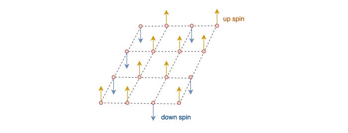
The distribution of the spin configuration for this lattice is:

We will introduce a few more concepts needed for later articles before the more important topic conditional random fields.

Moralization

A BN can be transformed into an MRF by changing the edge to un-directional and connecting the parents of a v-structure together.

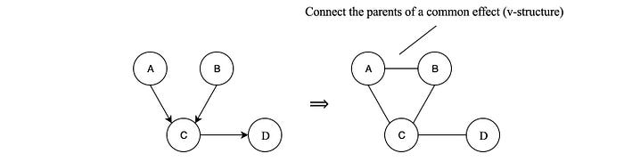
Moralization converts a BN into an undirected graphical model but it does not necessarily preserve all the conditional independence. For example, A ⊥ B is lost while A is not independent of B given C is introduced.

Shortcomings of MRF

Here are the shortcomings of MRF:

Computing the partition function Z is NP-hard in general, the use of approximation is usually required.
It is not a generative model. We cannot generate data/sample from this model easily.

In general, MRF can be more complex but computational intense. We may use BN first for simplicity unless it falls short on modeling independence.

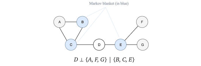
Markov blanket

Two nodes in an MRF are correlated if there exists a path between them containing all un-observed variables. So if all the neighbors of a variable are observed in an MRF, the variable is independent of any other un-observed variables. This is called the Markov blanket.

We can discover independence by studying how a graph is separated. Recall the limitation on BN, we can now demonstrate how to overcome our previous example with the MRF.

If B, D are observed, A and C are graphically separated and independent. If A, C are observed, A and C are independent. Therefore, we achieve the independence that the BN cannot achieve without adding more nodes.

We can prove that A and C are independent given B with probability theory.

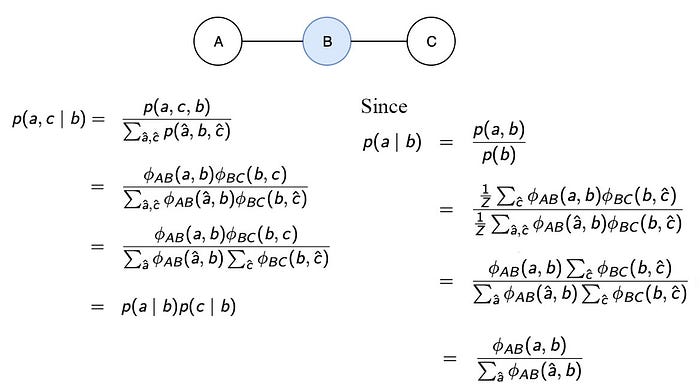
But this is awfully complicated for such a simple model. That is why we introduce the d-separated concept to make it much easier.

Graph separation is equilvalent to conditional independence. It is a much easier tool for discovering independence.

Conditional Random Fields

Previously, we are building a GM to model a joint distribution for p(x₁, x₂, x₃, …). Once this is built, we make all kind of possible queries using this joint probability. Nevertheless, in many ML problems, we are interested in some specific type of query only. For example, in supervised learning, the type of query is usually in the form of the conditional probability p(y|x) where y is the label and x is the observation. As discussed before, given some variables are observed, we can prune the graph further to simplify the model.

Alternatively, we can design the GM at the beginning with the idea that the evidence is known. The trade-off is it can answer a specify type of query only. Conditional random fields (CRF) are undirected graphical models that model the conditional distributions p(y|x) directly. CRF is a special case of MRF. Once the graphical structure is built, all the factorization, model training, and inferencing will be the same as MRF. Below is one possible design for CRF which the observation xᵢ is related to yᵢ only and yᵢ is also related to y in the neighboring step. Indeed, this is the Hidden Markov Model (HMM).

For example, with the observed x (“CAEE”), we want to auto-correct the spelling and predict y (“CARE”). This problem can be modeled with the conditional probability P(y|x) as:

As shown, the R.H.S. is the same as MRF. What we have done is simplify the GM according to what dependence is needed if x is observed. The following is the specific factorization for our CRF example (a.k.a. HMM).

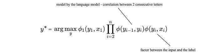
𝜙(yᵢ, xᵢ) rates the correlations of the label character i and the observed character i. As an example below, we can use the concept of the energy model to define 𝜙. The potential will be calculated with a linear model.

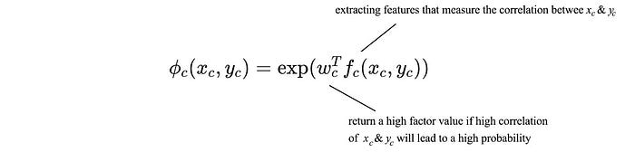
where f extracts the commonality between xc and yc before applying a linear regression with weight wc. Then, we apply an exponential function to the result.

HMM is one possible GM design for CRF. We can further generalize the model such that yᵢ is related to the whole observation X rather than a particular character. This model will be more complex but more powerful. The graph and the factorization will be rewritten as:

In this article, we discuss how to use a graphical model in representing a domain problem. However, we barely scratch the surface. We just give you a car manual and far away from knowing how to drive. In particular, how to make an inference and how to train the model. As always, when dealing with the probability models, many exact solutions are having NP complexity. So we will study in more detail on how to solve them efficiently.