RL — Actor-Critic Methods: A3C, GAE, DDPG, Q-prop

Value-learning, including Q-learning, is believed to be unstable when a large and non-linear function approximator, like the deep network, is used. This is a curse for many reinforcement learning training (RL). To address these problems, DQN applies experience replay and the target network. However, DQN handles discrete and low-dimensional action spaces only. For high-dimensional or continuous action spaces, finding the action with maximum Q-value requires complex optimization that seems impractical.

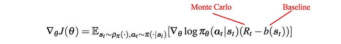
Policy Gradient method is popular. However, it has low sample efficiency and high variance. To reduce it, we can subtract the expected rewards with a baseline b. We can have different choices of b as long as it is not dependent on the model parameter θ. The optimal solution will be the same.

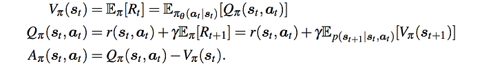
Often, we use the value function V(s) as a baseline. Then, we compute a new metric called the advantage function A which equals Q(s, a) minus V(s). Intuitively, we increase the chance of an action if it performs better than the average action.

The policy gradient is rewritten as:

Or

This new formularization introduces an actor, who determines the action based on a state. This can be modeled by a neural network NN parameterized by θ which supports actions for a continuous and high dimensional space also — something that DQN misses. In the next section, we introduce an NN called a critic to be used in computing A.
Actor-critic
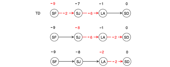
There are many ways to compute A. One possibility is taking an action step and observe the reward and the next state. So A approximately equals the reward plus the difference in the value function of the next state and the current state.

Here, we introduce another model V parameterized by 𝜙 below to estimate the value function of a state.

In this equation, we have two models: the actor which estimates the policy, and the critic which estimates the value function.
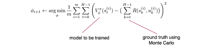
So how can we model V(s)? One good way is to use Monte-Carlo to find out the total rewards of a complete episode. Then, we use supervised learning to learn the critic model Φ.
Alternatively, we can apply the Temporal Difference TD concept to model V. Here is the formula with a 1-step lookahead.

In the equation below, we also add a regularization penalty to regulate the model 𝜙.

The Monte Carlo method is unbiased but with a high variance — a slight change in the sampled actions can change the result of a game completely. The TD method above is biased but low variance as it samples one action only. But the critic model is biased, at least in early training.
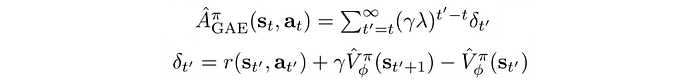
Generalized Advantage Estimation (GAE)
In practice, we can combine both Monte-Carlo and Temporal Difference TD methods. The following is a two-step lookahead with Temporal Difference TD.
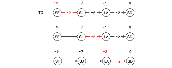
In the diagram below, we have a 1-step lookup, a 2-step lookup, and all the way to the Monte-Carlo method. Finally, we take a weighted sum to compute the expected rewards (underlined in red below).
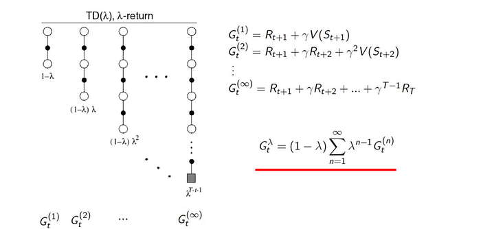
Let’s write it down formally. The advantage function for an n-step lookahead is:

The Generalized advantage estimation (GAE) is a hybrid combination of 1-step lookahead to the Monte-Carlo method. The hyperparameter λ ranges from 0 to 1. When λ=0, it is TD, and when λ=1, it is the Monte-Carlo method.
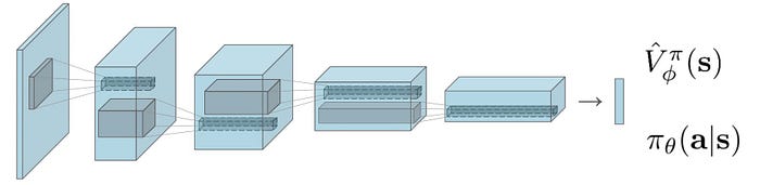
Actor-critic networks
Let’s recap. In the Actor-critic method, we have a deep network parameterized by θ to approximate the policy. This network is called the actor. We have a second network parameterized by Φ to approximate V. This network is called the critic. The Actor-Critic method is mainly a Policy Gradient method with the advantage function computed by the observed reward and the critic network. Here is the algorithm for the actor-critic algorithm that uses an online method.
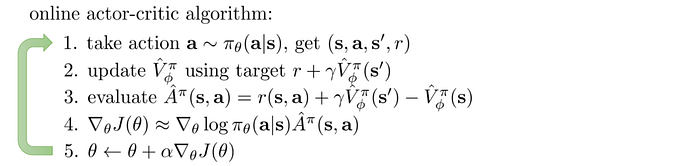
This should look similar to a Policy Gradient method. Policy Gradient utilizes gradient descent. It behaves nicely if the objective function is convex. However, Policy Gradient can suffer large variance. To overcome that, we can increase the batch size but it hurts the sample efficiency badly. By introducing a critic, it reduces variance and improves the sample efficiency at the cost of bias. To improve training stability, steps 2 and 4 above can be done with a batch of samples instead of one.
Asynchronous Advantage Actor-Critic (A3C)
Such batching processing can be done synchronously or asynchronously. A3C is an Actor-critic method that performs asynchronous parallel policy parameter updates.
Asynchronous actor-learners. A3C uses multiple asynchronous threads to learn the policy. Since threads are running asynchronous, each thread synchronizes its policy with the master at a different point in time. Hence, each thread explores a different part of the environment with slightly different policies. Actually, this helps the training with less correlation among samples. Deep learning is quite tolerable or welcomes errors (noises) in early training. In fact, lighting the accuracy requirements may help performance.

Previously, we use experience replay to improve RL performance. With this asynchronous calculation, experience replay is no longer needed. With multiple threads and the removal of experience replay, A3C produces better models in a shorter time.
k-step lookahead
A3C also applies TD with k-steps lookahead. Typically, it has k set to 5.

A3C algorithms
Below is the A3C algorithm. θ models the policy and θv models the value function V. Both θ and θv are implemented with the convolutional networks with parameters shared except the output layer. For θ, we use a softmax function to output the probabilities of actions. For θv, we use a linear layer to output a scalar value.
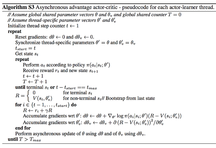
An entropy term on the policy is also added to the objective function. Entropy measures the randomness of the random variables. A deterministic policy has no randomness and therefore has zero entropy. The added term discourages the policy from collapsing to a deterministic policy too fast. This hurts exploration. So the extra term penalizes the model to be too sure of actions given specific states.

(β is a hyperparameter controlling the weight.)
Deep Deterministic Policy gradient DDPG
Absolute right can be absolutely wrong. So we have a stochastic policy to help us to explore in training. In DDPG, we have a deterministic policy. So, what does a deterministic policy may bring theoretically? The Q-value function can be learned through the Bellman Equation.

If we have a deterministic policy μ, we don’t need to have the second expectation function anymore. The equation can be simplified to:

In an on-policy RL method, like the vanilla Policy Gradient, the key focus is on improving the current policy. There is only one policy to determine what actions and what samples to use for the next training iteration. Whenever the policy is updated, we take new samples and they will be likely used once only. This hurt sample efficiency. For the equation above, the expectation function does not sample from μ. Indeed, Q can be fitted with all previous experience. In DDPG, previous samples are replayed to improve sample efficiency.
Applying chain rule, the policy gradient becomes:

DDPG is an off-policy method. There is more than one policy. Indeed, to fix the exploration limitation, a second policy is introduced. Gaussian noise is added to the current policy to determine the action to be sampled and executed.

The noise added helps exploration. Samples are stored in a buffer and randomly selected to train the critic and to refine the actor. This is the same as the experience replay in DQN. Also, DDPG uses the DQN’s target network concept. Here is the algorithm.
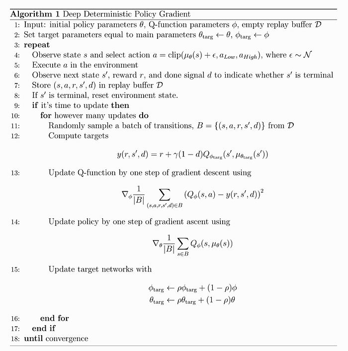
DDPG creates a deterministic policy for a high-dimensional continuous control space. We may argue that it is not exactly a deterministic policy. Nevertheless, empirical data show good performance with nice generalization to 20 different tasks without retuning hyperparameters.
Continuous & discrete space
Value learning methods require an extra step in determining actions from the value functions. It finds the optimal actions from the value functions for all possible actions. This may not be feasible if actions are in continuous or high-dimensional space. Therefore it is mainly for discrete control space. Policy gradient methods have an Actor. This separate model predicts what actions to take for a particular state. We can use a regressor and a classifier to model the continuous and discrete control respectively. Therefore, it works for both spaces. However, since actions are sampled from a deterministic policy, DDPG is for continuous control space only. For instance, it cannot handle actions with a bimodal distribution.
Q-Prop
Q-Prop is another Actor-critic method. In previous approaches, we introduce TD learning to reduce variance at the cost of bias. Q-Prop reduces the variance of gradient calculation without adding bias using the concept of control variate. This algorithm is relatively complex. So we will give an overview with jumping steps. Please refer to the paper for more details.
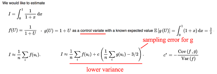
Control variate
Let say we want to calculate I expressed as an integral of f(U) below. This can be done by sampling the value of U and take the average of f(U).

However, the estimation varies depending on the sampled values for U. Control variate is a technique to reduce the variance of this estimation. First, we establish a function g that is related to f. We choose g such that its expected value can be calculated analytically. By sampling U, we estimate I. But we also compute the corresponding g(U) and calculate how the values deviate from the expected g. We recalibrate our estimation of I by introducing a second term showing this deviation.
Adaptive Q-Prop method
Now, we apply the same concept to solve the high variance problem in the policy gradient.
Let’s summarize something we already learned first. The following equation computes the Policy Gradient with Monte Carlo. It is unbiased.
We can use V as a baseline to reduce variance and the advantage function A is:
The idea of the Actor-critic is to fit the actor and critic model:

With the policy gradient calculated as:

So far, we have just repeat what we learn.
Let’s subtract and then add an arbitrary function f into the policy gradient.
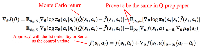
where we estimate any arbitrary function f with the Taylor series.

And

So, let’s choose what is f.

Therefore,

where

In Policy Gradient, we use A instead of Q. So let’s make the same change here. The new formularization of the Policy Gradient becomes:
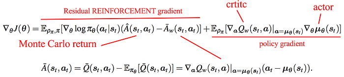
It composes of the residual REINFORCE gradient and the regular policy gradient. Q is the critic model that we learn.
Q-Prop is a Monte Carlo policy gradient estimator with a special form of a control variate. To reduce the variance, we introduce η(s) to scale some of the terms.
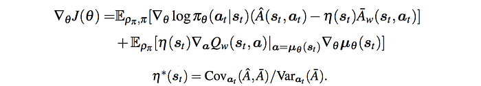
The optimal state-dependent factor η(s) can be computed per state using η* above. η* provides maximum reduction in the variance. The policy gradient computed in this form is called the adaptive Q-Prop method.
Conservative and Aggressive Q-Prop
η* has a high variance also. Therefore the Conservative Q-Prop is proposed as

Which turns off the control variate when  and Ā are negatively correlated, i.e. when the critic is very bad. In Aggressive Q-Prop, it is set to

Conservative Q-Prop will achieve more stable performance than the standard and aggressive variants. Here is the algorithm for the Adaptive Q-prop. It is a mixture of policy gradient and actor-critic.

Demonstrations
Here are the demonstrations using GAE and asynchronous actor-critic methods.