RL — Conjugate Gradient
We use the Conjugate Gradient (CG) method to solve a linear equation or to optimize a quadratic equation. It is more efficient in solving those problems than the gradient descent.

where A is symmetrical and positive definite.

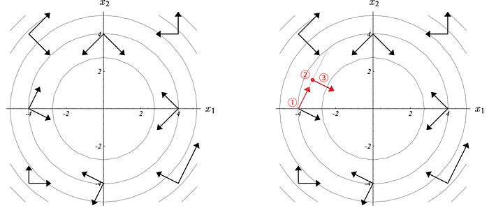
In a line search, we determine the steepest direction of ascent and then select the step size. For example, in the gradient ascent method, we take a step size equals to the gradient times the learning rate. For the figure on the left below, the deepest direction according to the gradient contour (the dotted eclipse) is moving right. The next move may go up and slightly to the left according to the steepest gradient at the current point. But isn’t that undo part of the progress in the first move if we turn left slightly?

The conjugate gradient method is a line search method but for every move, it would not undo part of the moves done previously. It optimizes a quadratic equation in fewer step than the gradient ascent. If x is N-dimensional (N parameters), we can find the optimal point in at most N steps. For every move, we want a direction conjugate to all previous moves. This guarantees that we do not undo part of the moves we did. In short, if x is 4-dimensional, it should take at most 4 moves to reach the optimal point.

- We start the ascent in one particular direction.
- We settle down in the optimal point for that direction.
- We find a new direction dj which is A-conjugate to any previous moving directions di.
Mathematically, it means any new direction dj must obey the A-conjugate with all previous direction di:

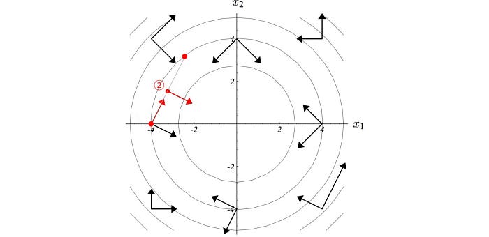
where A is the matrix in the quadratic equation. Here are some other examples of A-conjugate vectors in 2-D space.

The A-conjugate vectors are independent of each other. Hence, N A-conjugate vectors can span a space of N dimensions.

The key part of the CG method is to find α and d.
CG Algorithm
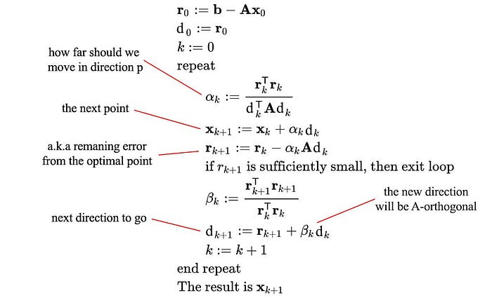
But let’s have a preview of the algorithm first. We start with a random (or educated) guess for the solution on X (Xo) and calculate the next guess X1 with α and d.

d is the direction (the conjugate vector) to go for the next move.
Let’s see how it works in details. First, we define two terms:
- e is the error between the current guess and the optimal point.

- r measures how far we are from the correct value b (Ax=b). We can view r as the error e transformed by A to the space of b (how far Ax is from b).

From,

We can derive:

Our next point is computed as (which α is a scalar and d is the direction):

In order for the future direction not to undo progress from the previous directions, let’s try d and e to be orthogonal. i.e. the remaining error after taking this step should be orthogonal to the current direction. This makes sense if the remaining moves should not undo part of the move we just did.

α depends on e which we don’t know its value. So instead of orthogonal, let’s try another guess. A new searching direction should be A-orthogonal with previous one. The definition of A-orthogonal is:

To fulling these conditions, the next point xi has to be the optimal point in the search direction d.


Using the A-orthogonal requirement, α is computed as:

Proof
We will not go through the proof. But for those interested:
en.wikipedia.org/wiki/Derivation_of_the_conjugate_gradient_method
