RL — Inverse Reinforcement Learning
It is a major challenge for reinforcement learning (RL) to process sparse and long-delayed rewards. It is difficult to untangle irrelevant information and credit the right actions. In real life, we establish intermediate goals for complex problems to give higher-quality feedback. Nevertheless, such intermediate goals are hard to establish for many RL problems.
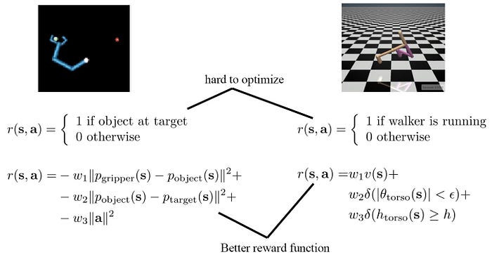
This insight leads to the need for a smooth reward function to trace the effect of actions. We want to avoid a reward function with vanishing or exploding gradients. The cost function in the left gives no direction on where to search unless it is at the edge of the optimal point. For this type of cost function, no optimization method can do better than a random search. The cost function in the right is much smoother and gives quality information everywhere on where to search next.

Let’s consider a gripper that grips an object to a target location. We can give a reward when the object reaches its target position. But the long delay makes it hard to find the solution. Alternatively, a reward function can measure the distance between the object and the gripper as well as the target location. This alternative approach gives better and more frequent feedback. Nevertheless, modeling such reward functions precisely and explicitly to a wide range of RL problems is hard.
What is Inverse Reinforcement Learning?
Many RL methods focus on the model or the policy. Model a better reward function is what inverse reinforcement learning addresses.

In Policy Gradient methods, the rewards are observed to adjust the policy. Nevertheless, the observed rewards used are often sparse with long delays. In Model-based RL, a small error in the model leads us to extremely different rewards.
Conceptually, our goal is to learn the intent that can provide better guidance along the process. But, like other deep learning (DL) or machine learning problems, it is hard to model them explicitly. But we can borrow a page from the supervised learning in DL. We can fit a reward function using expert demonstrations. Once a reward function is fitted, we can use Policy Gradient, Model-based RL or other RL to find the optimal policy. For example, we can compute the policy gradient using the reward function instead of sampled rewards. With the policy gradient calculated, we optimize the policy towards the greatest rewards gain.
In inverse reinforcement learning, the challenge is can we model the rewards better to make better decisions.

In a nutshell, given an expert demonstration, we model a reward function. We then use that to derive a better policy.

However, in many RL problems, finding a label for supervised learning is not feasible. And like many DL problems, the mentioned approach can be extremely sample-inefficient. So one of the goals in inverse RL is to fit such models with fewer demonstrations if those are expensive.
For example, in the video below, the researcher is holding a robot arm to place dishes onto a dish rack. After 20 demonstrations, the PR2 robot can place the dish onto a target slot on its own. In the process, PR2 learns the reward function and performs Policy optimization through the learned reward function.
Maximum Entropy Inverse RL (MaxEnt)
So how can we model a reward function r? We start by creating a reward model parameterized by ψ.

Since it is hard to label the rewards, we model the likelihood of a trajectory. In Policy Gradient, we define an objective function in maximizing the probability of a trajectory based on the policy. In inverse RL, we maximize such a probability based on the reward instead. The probability of the expert demonstration is proportional to the exponential of the reward. Then, we normalize this score with the scores of all possibilities to compute the probability.

The higher the rewards, the more likely a trajectory would be. Similar to the Policy Gradient, we can compute its gradient (a.k.a. reward gradient) relative to the reward parameters ψ to learn the reward model. But since there are infinite alternative trajectories, it is intractable to compute the exact value for the denominator. Instead, we will estimate the integral with the expected value, i.e. 𝔼(exp(rewards)).

Furthermore, we can frame the expected value as to how frequently we land in a state multiplied by its expected rewards. To fit the reward model, we maximize the likelihood of the expert demonstrations above with the corresponding reward gradient as (with proof later):

So how can we find the visitation frequency p(s|ψ)? An optimal policy

can be computed from the reward function, say using Policy Gradient.

Once we compute the policy, we can estimate the visitation frequency of a state providing that we know the system dynamics (details in the next section).

Let’s detail the step a little bit more. We initialize a reward model ψ randomly or with an educated guess. We also have experts performing the tasks as demonstrations D. Based on the assumed reward model, we solve what is the optimal policy (say using Policy Gradient). Then, we compute the state visitation frequencies. Now we are ready to compute the reward gradient and use it to refine the assumed reward model. We continue the iteration as both the policy and the reward model will continue to improve and converge.

Reward Gradient Proof (Optional)
Let’s prove the reward gradient. Here is the notation used in this section.

Recall the probability of a trajectory is defined as:

Our key focus is on how to compute the partition function. We define the objective as maximizing the log probability of a trajectory:

The objective function is

where M is the number of demonstration trajectories. After taking its derivative, the gradient can be expressed in terms of state visitation frequency p:
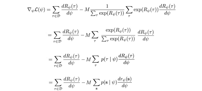
The visitation frequency can be calculated from the system dynamics and the policy:
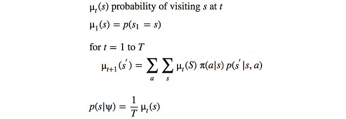
So once the visitation frequency is computed, we can use gradient ascent to optimize the objective.
Maximum Entropy Inverse RL has a few strong assumptions. First, the system dynamics are known and we have limited states so it is not too hard to compute the state visitation frequency. Unfortunately, this may not be true for many RL tasks.
Guided Cost Learning (GCL)
How can we handle unknown system dynamics? If we do not know the dynamics, we cannot compute the state visitation frequency p.

GCL formulates a sample-based approximation for MaxEnt IOC to estimate the partition function Z.

In this section, we will change some of the notations. We will use the cost function instead of the reward function and divide the cost by the number of samples. The cost function will be parameterized as θ.
The first term in the objective function is calculated from the trajectories in the expert demonstration. For the second term, we apply the importance sampling concept to calculate

Importance sampling samples trajectory τ and observes the output f(τ) to calculate expected values.

Let’s say the sampling distribution to estimate 𝔼 for τ will be q(τ). So how q may look to estimate 𝔼 better?
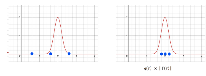
As graphically shown above, q will be better off to be proportional to:

i.e., we can focus on likely trajectories and ignore the unlikely ones for the cost-expectation estimation. For details on the importance sampling, please see this article.
The second term will become:

In short, if we sample trajectories proportional to the reward, the better will be our estimate. Using this formulation, the partition function will be estimated without the knowledge of system dynamics.
Now we are ready to put everything together. Besides a reward model, we fit a policy model also — instead of solving it every time from an assumed reward model.
The key concept is we use expert demonstrations to compute the likelihood of expert demonstration and use trajectories samples from the policy (a.k.a. q) to estimate the likelihood of all possibilities (the partition function).
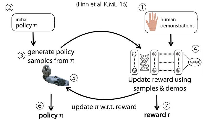
1. We collect a set of human demonstrations.
2. We initialize a controller π(a|s) (a.k.a policy).
3. We run this controller on the robot and observe the sampled trajectories.

4. Using these samples and the human demonstrations, we calculate the reward gradient to update the reward model.

5. Similarly, using the Policy Gradient method, we refine the policy model using the updated reward function.
6. As the policy is updated, it gets better in sampling trajectories with higher rewards.
7. A better policy gives a better estimate for (4) and therefore the reward function is getting better also.
As we run it iteratively, we improve the reward function and the policy in an alternative step. The improved policy will create trajectories with higher rewards and therefore our reward gradient will be more accurate to refine the reward model.
In contrast to Maximum Entropy Inverse RL, we do not need to fully optimize the policy in step (5). We can take a single Policy Gradient step.
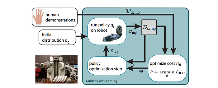
Finally, this is the algorithm.


More details can be found in the GCL paper.
Dish experiment
Here are the experiment settings in the video. This is quoted from the Guided cost learning paper directly:
The dish placing task has 32 dimensions (7 joint angles, the 3D position of 3 points on the end effector, and the velocities of both). Twenty demonstrations were collected via kinesthetic teaching on nine positions along a 43 cm dish rack. A tenth position, spatially located within the demonstrated positions, was used during IOC. The input to the cost consisted of the 3 end effector points in 3D relative to the target pose (which fully define the pose of the gripper) and their velocities. The neural network was parametrized with 1 hidden layer of dimension 64 and a final feature dimension of 100. Success was based on whether or not the plate was in the correct slot and not broken.
GAN (optional)
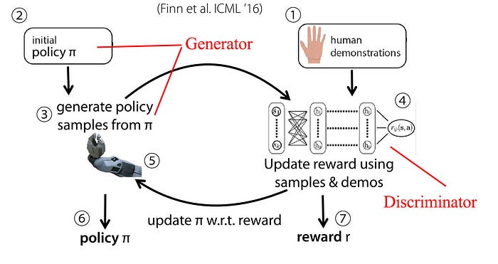
GAN (Generative Adversarial Networks) uses a generator to generate data from scratch. A discriminator is trained to distinguish between real and generated data. We also backpropagate the information back to the generator to let it know what should be improved. We knock the generator and the discriminator into a fierce competition so the discriminator can distinguish the slightest difference while the generator can generate undetectably generated data.

Guided cost search has a close resemblance to GAN. In fact, they can show that their objective function in training the model is either the same or similar to GAN. In short, the policy π tries to generate actions similar to experts while the reward model tries to discriminate between human and computer actions.
Credits and references
UC Berkeley Reinforcement learning Bootcamp
