RL — Model-based Reinforcement Learning
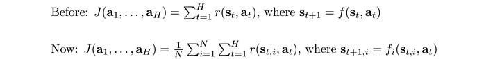
Reinforcement learning RL maximizes rewards for our actions. From the equations below, rewards depend on the policy and the system dynamics (model).

In Model-free RL, we ignore the model. We depend on sampling and simulation to estimate rewards so we don’t need to know the inner working of the system. In Model-based RL, if we can define a cost function ourselves, we can calculate the optimal actions using the model directly.
RL can be roughly divided into Model-free and Model-based methods. In this article, we will discuss how to establish a model and use it to make the best decisions.
Terms
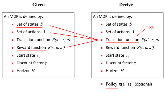
Control theory has a strong influence on Model-based RL. Therefore, let’s go through some of the terms first.
In reinforcement learning, we find an optimal policy to decide actions. In control theory, we optimize a controller.

Control is just another term for action in RL. An action is often written as a or u with states as s or x. A controller uses a model (the system dynamics) to decide the controls in an optimal trajectory which is expressed as a sequence of states and controls.

In model-based RL, we optimize the trajectory for the least cost instead of the maximum rewards.
Model-free RL v.s. Model-based RL
As mentioned before, Model-free RL ignores the model and care less about the inner working. We fall back to sampling to estimate rewards.

We use Policy Gradients, Value Learning or other Model-free RL to find a policy that maximizes rewards.

On the contrary, Model-based RL focuses on the model.

With a cost function, we find an optimal trajectory with the lowest cost.

Known models
In many games, like GO, the rule of the game is the model.

In other cases, it can be the law of Physics. Sometimes, we know how to model it and build simulators for it.

Mathematically, the model predicts the next state.

We can define this model with rules or equations. Or, we can model it, like using the Gaussian Process, Gaussian Mixture Model (GMM) or deep networks. To fit these models, we run a controller to collect sample trajectories and train the models with supervised learning.
Motivation
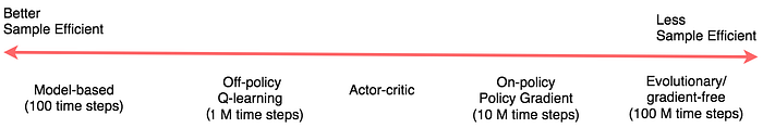
Model-based RL has a strong advantage of being sample efficient. Many models behave linearly at least in the local proximity. This requires very few samples to learn them. Once the model and the cost function are known, we can plan the optimal controls without further sampling. As shown below, On-policy Policy Gradient methods can take 10M training iterations while Model-based RL is in the range of hundreds. To train a physical robot for a simple task, a Model-based method may take about 20 minutes while a Policy Gradient method may take weeks. However, this advantage diminishes when physical simulations can be replaced by computer simulations. Since the trajectory optimization in Model-based methods is far more complex, Model-free RL will be more favorable if computer simulations are accurate enough. Also, to simplify the computation, Model-based methods have more assumptions and approximations and therefore, limit the trained models to fewer tasks.
Learn the model
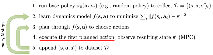
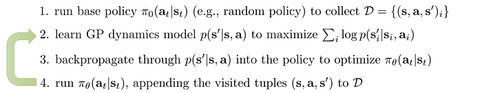
In Model-based RL, the model may be known or learned. In the latter case, we run a base policy, like a random or any educated policy, and observe the trajectory. Then, we fit a model using this sampled data.
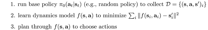
In step 2 above, we use supervised learning to train a model to minimize the least square error from the sampled trajectory. In step 3, we use any trajectory optimization method, like iLQR, to calculate the optimal trajectory using the model and a cost function that say measure how far we are from the target location and the amount of effort spent.
Learn the model iteratively
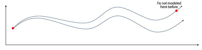
However, it is vulnerable to drifting. Tiny errors accumulate fast along the trajectory. The search space is too big for any base policy to cover fully. We may land in areas where the model has not been learned yet. Without a proper model around these areas, we cannot plan the optimal controls.
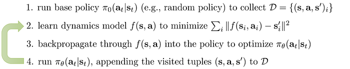
To address that, instead of learning the model at the beginning, we continue to sample and fit the model as we move along the path.
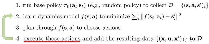
So we repeat step 2 and step 4 and continue collecting samples and fitting the model around the searched space.
MPC (Model Predictive Control)
Nevertheless, the previous method executes all planned actions before fitting the model again. We may be off-course too far already.

In MPC, we optimize the whole trajectory but we take the first action only. We observe and replan again. The replan gives us a chance to take corrective action after observed the current state again. For a stochastic model, this is particularly helpful.
By constantly changing plans, we are less vulnerable to problems in the model. Hence, MPC allows us to have models that are far less accurate. Here is a video on how a model is trained under this concept.
(source)
Backpropagate to policy
The controls produced by a controller are calculated using a model and a cost function using the trajectory optimization methods like iLQR.
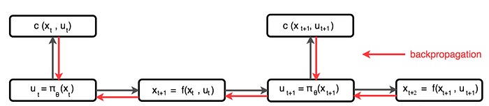
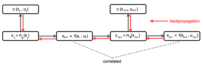
However, we can also model a policy π directly using a deep network or a Gaussian Process. For example, we can use the model to predict the next state given an action. Then, we use the policy to decide the next action, and use the state and action to compute the cost. Finally, we backpropagate the cost to train the policy.
PILCO
Here is the PILCO algorithm of training a policy directly through backpropagation.
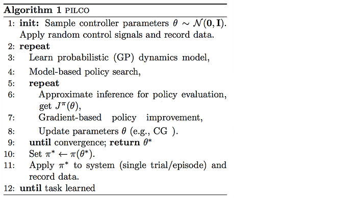
However, consecutive states in a trajectory are highly correlated. Backpropagation functions with correlated values often lead to vanishing or exploding gradients. So its promise is limited.
Global Model
What kind of models can we use to represent the system dynamics?
One possibility is the Gaussian Process. The intuition is simple. If two inputs are similar, their output should be similar too. For two data points, if one is closer to a known training data, its prediction is more certain.
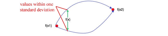
Say, we sampled two data points x1 and x2 with observed values f(x1)=150 and f(x2)=200 respectively. Can we determine the likely values of f(x) for x1<x<x2? The plot above shows these possible values of f(x) within one standard deviation. As shown, the middle point between x1 and x2 should have the highest uncertainty about its value. The output of data points, like f¹and f², can be modeled as a Gaussian Distribution in the following form.


where 175 is the mean of f. K is the covariance matrix with each elementᵢⱼ measures the similarity between input xᵢ and xⱼ. For details on how to calculate K, please refer to here.
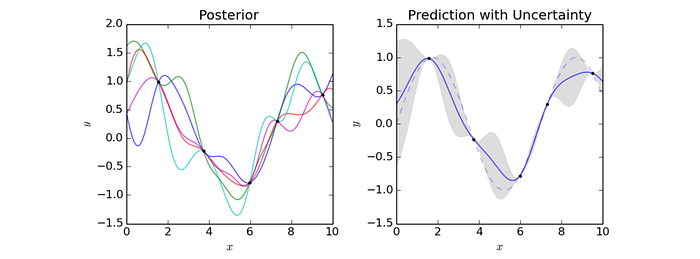
As another example, the right figure below samples the output of 5 data points. The graph plots the predictions using the Gaussian process. The blue line represents the means and the shaded area represents values within one standard deviation (SD). So for input x=5, the prediction within one SD is between -1.1 to -0.4 with mean about -0.7.
Here is the algorithm of the policy search using a Gaussian Process (GP) model:
Another possibility is the GMM. Gaussian Mixture Model is a mixture of K Gaussian distributions. We assume the model has k most likely outcomes and we weight each possibility according:

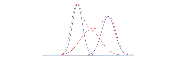
To identify those k Gaussian distributions, we use Expectation-Maximization (EM) to cluster the sample data into k clusters (modes) that each represented by a mean and variance.
Deep network
Finally, we can also use a deep network.
Global model
Previously, we model the dynamics with a global model. If the dynamic is complex, we need a more expressive model like the deep network. But it requires a lot of samples to train it. If we land in space which is not yet trained properly, the model can be erroneous and lead us to bad actions that destroy the progress of the training.
Local Model
Alternatively, we can adopt an on-demand approach in developing models locally when we need it.

The local model is Gaussian distributed with linear dynamics.

The parameters for the linear dynamics is computed as:

Next, we will see how we train and use the controller to take action.
Controller
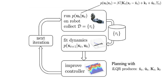
We run the controller p on the robot and observe the trajectory. With the collected samples, we can fit the model locally by estimating the derivative using samples.

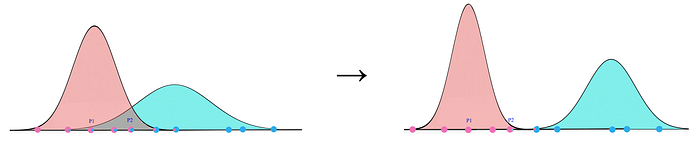
However, the potential error increases as we move away from the trajectory where the local model is developed. Hence, we add a constraint to make sure the trajectory optimization is done within a trust region. In short, we will not take action outside this region which we cannot trust the optimization result.

This trust region is determined by the KL-divergence which measures the difference between the new controller and the old controller. If the trajectory is too different from the sampled one, we may get too aggressive and the calculated value can be too far away from the real value.

So what controller should we use? It will be too boring if the controller explores the same action over and over again for the same state during training. The repeating samples provide no new information to make the model better. Hence, we use a linear Gaussian controller to explore actions better. (linear dynamic with a Gaussian distributed output actions)
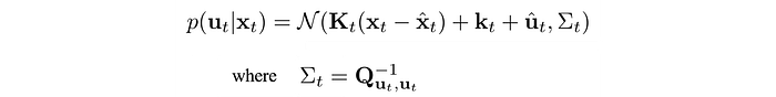
and Q is the cost function:

Σ is large when the cost Q is small. So we allow the exploration to go off-course more if the estimated cost is low. So how can we find a new controller in minimizing cost given the controller change is within a trust region?

Before solving that, we need to check out some of the properties of the KL-divergence between the new and the old controller. This will involve some maths but it should be easy to follow or feel free to browse through them quickly.
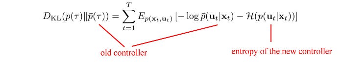
KL-divergence
We want to establish:
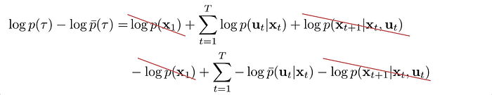
First, we expand the distribution of the trajectory using the new and the old controller:

(Note: both trajectories have the same initial and final state.)
Let’s compute the log term below first which is part of the KL-divergence definition:
KL-divergence is defined as:

Therefore, the corresponding KL-divergence is:

Dual Gradient Descent
Next, we need an optimization method that works with constraints.

DGD is our choice. Let’s have a quick summary here. For those want more details, you can read DGD later. First, we need to find its Lagrangian 𝓛 and the Lagrange dual function g which is defined as:
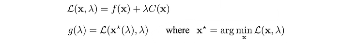
Then the optimal x* of our objective can be solved by:

Intuitively, we start with some random value of λ and find the corresponding optimal values of 𝓛 using an optimization method. In our context, this will be a trajectory optimization method like LQR. Without proof here, g (i.e. 𝓛(x*, λ)) is actually the lower bound of our objective. So we want to move along g such that it gets higher and closer to our objective function. That is what steps 2 & 3 do which use gradient descent to move λ towards the steepest direction in increasing g. Then, with the new λ, we compute a new lower bound g. As we keep the iteration, we will find λ in which the maximum of g touches the minimum value of the objective function.
Model-based RL with local model
Again, our objective is:
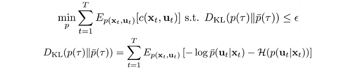
We will use LQR to optimize step 1. LQR is quite complicated but for this context, you just need to know LQR is a trajectory optimization method. You can read LQR later if you want more.
The Lagrangian for our objective is:
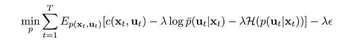
We divide the objective by λ and create a new surrogate cost function
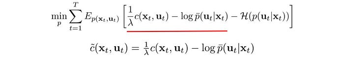
Here is the objective with the Lagrangian:

As explained in a previous article, LQR solves:

With a Linear Gaussian controller,

Then, we can apply LQR to minimize

This looks almost the same as our objective but the equation above uses the original cost function c. So to solve our objective, we can follow the same procedure but use our surrogate cost function instead of c.
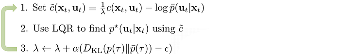
Optimize trajectory with a local model
This is the final algorithm:
Planning
We can also use planning to generate simulated experience and use them to fit the value functions or the policy better.
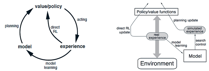
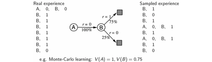
The difference between learning and planning is one from real experience generated by the environment and one from simulated experience by a model. We use the real experience to fit the value function. We build a model of the transition and sample experience from it. Later, we can fit the value function again with the sampled experience. This improves sample efficiency because sample data are reused and it produces a more accurate value for V.
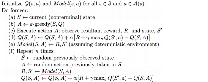
Dyna-Q Algorithm
Here is the Dyna-Q algorithm which used the sampled data and the model to fit the Q-value.
Let’s discuss another example of using a model for a Model-free method. The variant for Policy Gradient is usually high.

But it can be reduced by averaging out from a large sample. This is expensive if physical simulations are needed. But we have a model, we may be able to generate the needed data from the model.
Overfit
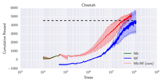
In a Model-based method, we use a relatively small amount of training samples because of the computation complexity. In addition, we can use a deep network to model system dynamics. Nevertheless, we need to keep the capacity of the model small. Otherwise, it will be overfitted. Such an overfitted model will make bad decisions. However, this simple model also limits the maximum rewards. For example, in the Cheetah task below (a task to teach a simulated Cheetah to run), a Model-based method can not reach a total reward beyond 500. To reach higher, we need a more complex model with more training data. A more feasible solution is using a Model-based method to train a simple model. Then we use this model to initialize a model-free learner and use model-free training to push the expected rewards further up.
Model-based RL with ensembles
Another alternative is using an ensemble method based on the idea that independently trained models do not make the same mistakes and many weak learners can be combined to make good decisions. So instead of training one model, we can use different seeds to train many different models.
In planning, given a sequence of actions, we can determine the state transitions from each model and find out the reward. The reward of such an action sequence equals the average rewards using all these models.
Distillation
Overconfidence always kills. When we label our data, we make it as a definite answer. But in reality, this is less definite in reality. For example, the letter below is a 1 or a 7.

One problem in ensemble methods is the computation complexity increases by k times with k models. In distillation, we plan to match its performance but use one model only during inference. We still train the ensemble models and we use the prediction of the ensemble as a soft label.

where T is the tunable parameter Temperature and zᵢ is the logit output of the ensemble. We train another model with the intention to match the value of this soft label instead. Intuitively, we create a new model on what this ensemble may predict.
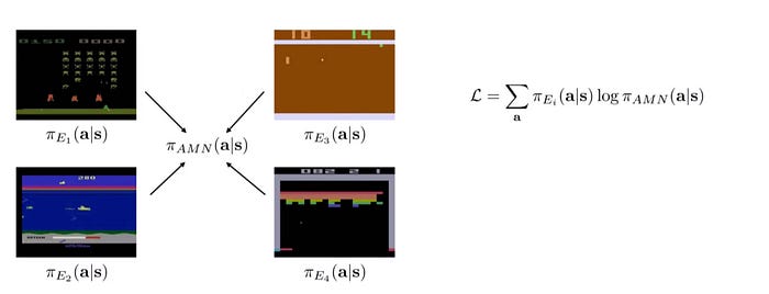
This strategy can be applied to create a single policy for multiple tasks. For example, we can train a policy for each Atari game below. Once these policies are trained, we will use supervised learning to match what these policies may predict. The objective function is simply a weighted log probability of the unified policy and weights derived from different individual policies.
Thoughts
Instead of fitting a policy or a value function, we develop a model to understand the inner workings better. Knowing how things work, we end up with fewer required samples which is the key selling point when the physical simulation is expensive. Here, we discuss the basic of the model learning. But I wish it is that simple. Model learning can be very hard and not generalize well for other tasks. Learning directly for raw images is difficult when information is all tangled. Can we deploy the solution that is economically feasible? Stay tuned for these questions for more in-depth Model-based RL methods in later articles.
