RL — Policy Gradients Explained (Part 2)
In the first part of the Policy Gradients article, we cover the basic. In the second part, we continue on the Temporal Difference, Hyperparameter tuning, and Importance Sampling. Temporal Difference will further reduce the variance and the importance sampling lays down the theoretical foundation for more advanced policy gradient methods like TRPO and PPO.
Temporal difference TD
Next, consider you are a driver who charges your service by hours. So the value function V(s) measures how many hours to get to your final destination. We can bootstrap the value function from traveling from San Francisco to San Diego as:

which it assumes it takes 1, 6 and 1 hours of travel for each segment respectively.
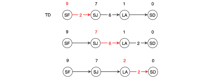
Let’s sample our experience with a Monte Carlo rollout. In the example below, the trip takes 2, 6 and 2 hours for each segment respectively. The calculated V(SF) becomes 10 now.

Instead of Monte Carlo, we can use the temporal difference TD to compute V. In a 1-step lookahead, the V(S) of SF is the time taken (rewards) from SF to SJ plus V(SJ). So here is the result of the same sampled trajectory.

This scheme has a lower variance because we are looking into fewer actions. However, at least in the early training, it is highly biased as the V values are not accurate. As we progress, the bias in V will lower.
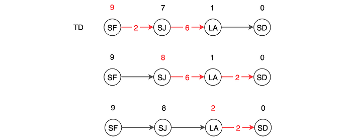
Here is the result with 2-step lookahead.

Let’s write down the math. For a one-step lookahead, V is

The temporal difference becomes

We can compute the Q function with a similar concept.

So which one do we use in calculating the policy gradient?
Generalized advantage estimation (GAE)
An n-step look ahead advantage function is defined as:

In GAE, we blend the temporal difference results together. Here are different advantage function with 1 to k-step lookahead.

The final advantage function for GAE is

where λ is a hyperparameter from 0 to 1. When λ is 1, it is Monte Carlo. When λ is 0, it is TD with one step look ahead.

Now, we have the formula to blend Monte Carlo and TD together. But we still have not answered what λ to use. This will be answered next in hyperparameter tuning.
Hyperparameter tuning
What are the hyperparameter values for the reward discount rate γ and λ?
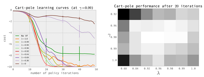
λ blends TD results with Monte Carlo to reduce variance. As λ decreases from one to zero, we weight heavier towards the TD than Monte Carlo. TD reduces variance but it increases bias. We are not using the exact result from playing the whole trajectory in computing the rewards and therefore the bias increases. In practice, we want mainly Monte Carlo result with some minor help from TD. As shown below in the figure on the left for one of the toy experiment, the cost drops as we have λ closer to one but not exactly one. So we should focus on Monte Carlo with little TD learning.

In many RL problems, the rewards obtained in the future is as good as the rewards now. The discount rate γ can set to one for no discount. However, in many algorithms, like Actor-critic algorithm, the variance in the Q estimation (the critic value) decreases if γ is smaller than one. This helps the models to learn much better even the problem itself does not ask for it.
In the toy experiment demonstrated above, it achieves the best performance (the brighter the better in the figure above) when γ is 0.98 and λ is 0.96. These parameters need to be tuned and hopefully, this section gives you some pointers.
On-policy learning v.s. off-policy learning
PG that we described is an on-policy learning. We refine the current policy and use the same policy to explore and to collect samples to compute the policy gradient.

On-policy learning has poor sample efficiency. Next update needs to recollect new samples again using the new policy to compute the policy gradient. Old samples collected are not reusable. For a trajectory with hundreds of moves, this is awfully inefficient for just a single policy update.
Alternatively, the rewards of a trajectory can be computed using importance sampling. In importance sampling, the expected reward can be computed with a different policy and later recalibrated by the distribution ratio of τ (underline in red below).

So the expected rewards can be estimated from samples collected from previous policy. This opens the door of not refreshing the collected samples whenever a policy is changed. But it has its own limitations.
Importance sampling
But let’s look into how importance sampling is related to policy gradient first. Can we derive the Policy Gradient using importance sampling?

This is the same result that we derive the policy gradient before.
Based on that, we can express our objective using importance sampling. The policy gradient becomes:

Again, we will deal with a chain of multiplication that may explode or shrink to zero.
Let’s rework on the objective function again:

Applying importance sampling, it becomes:

If we can constraint how far we change the policy, we can ignore the term cross out above. i.e. the probability distribution of states between two similar policies should be close to one. Hence, the objective can be formulated as

with an added constraint that the new policy cannot be different from the old policy by δ (measured with divergence). And we can improve and refresh the objective iteratively to find the optimal policy.
Why do we formulate the problem in yet another way using the importance sampling? In RL, the input training samples change alone the course of training. As we know better, we search a different part of the space. The tradition optimization in deep learning like gradient descent assumes the data distribution for input is relatively constant. However, RL breaks this assumption and makes learning rate tuning very hard.
The importance sampling concept provides a foundation for more advanced Policy Gradient methods including TRPO and PPO. The added constraint provides us with a guideline of how far we can change the policy before our calculation will be too far away from the current policy and we can not trust the calculation anymore. This trust region helps us not to take over-optimistic actions that hurt the training progress. To detail the concept, it needs more explanation and therefore we will reserve the discussion in separate articles.
More thoughts
In Q-learning, we try out different actions from a state and figure out how good (the value of Q) in taking those actions. Does Curry try our different poses and measure how good they are? Or he starts with some pose and evolves them gradually (Just like the Policy Gradient). We will not have the answer for you. There is no theoretical reasoning to claim whether Q-learning or Policy Gradient is better. In practice, we work with limit resources and different approaches may favor different RL tasks. But Policy Gradient is obviously one intuitive and popular way to solve RL problems. This is how a human may make decisions and the RL training is more interpretable.
However, Policy Gradient has high variance and bad sample efficiency. To combat the variance problem, we need a larger batch of samples to compute each policy gradient. We can compute a baseline to reduce the variance. To balance between bias and variance, GAE mixes Monte Carlo and TD learning which provides us a mechanism to tune the training using different tradeoffs. Tweaking learning rates for PG is very hard. Consider using more advanced optimization like ADAM or RMSProp.
Advanced Policy Gradient Methods
Nevertheless, Natural Policy Gradient becomes a more popular approach in optimizing the policy. It discourages making too aggressive moves that turn out to be wrong and destroy the training progress. Conceptually, it was done by taking moves only within a trust-region distance. In short, don’t make policy change so big that the calculation becomes not reliable enough to be trusted. But the new approach is a second-order optimization that suffers badly in complexity and does not scale well for large models. TRPO is introduced to remove the necessity of computing the expensive inverse of the Fisher Information Matrix FIM. But it is still not enough since computing the FIM still requires a lot of sampling. Can we relax the requirement from the Natural Policy Gradient so we don’t need to perform a second-order optimization? PPO responds by only imposing a soft constraint on the policy change so it can use the regular gradient ascent method in optimizing the object. Here is a quick summary of the trends in Policy Gradient. Stay tuned in the deep reinforcement learning series articles for each advanced method.
