RL — Trust Region Policy Optimization (TRPO) Explained

Policy Gradient methods (PG) are popular in reinforcement learning (RL). The basic principle uses gradient ascent to follow policies with the steepest increase in rewards. However, the first-order optimizer is not very accurate for curved areas. We can get overconfidence and make bad moves that ruin the progress of the training. TRPO is one of the most quoted papers in addressing this issue. However, TRPO is often explained without the proper introduction of the basic concepts. In Part 1 here, we will focus on the challenges of PG and introduce three basic concepts: MM algorithm, trust region, and importance sampling. But if you are comfortable with these concepts already, scroll down to the end for Part 2 in detailing TRPO.
Challenges of Policy Gradient Methods (PG)
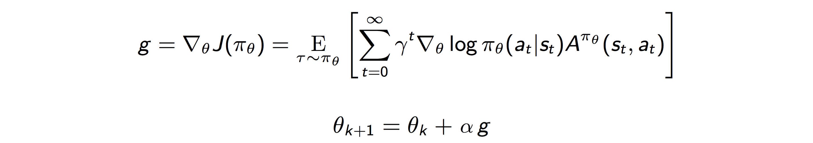
In RL, we optimize a policy θ for the maximum expected discounted rewards. Nevertheless, there are a few challenges that hurt PG performance.

First, PG computes the steepest ascent direction for the rewards (policy gradient g) and update the policy towards that direction.

However, this method uses the first-order derivative and approximates the surface to be flat. If the surface has high curvature, we can make horrible moves.

Too large of a step leads to a disaster. But, if the step is too small, the model learns too slow. Picture the reward function as the mountain above. If the new policy goes too far, it takes actions that may be an inch too far and fall off from the cliff. As we resume the exploration, we start from a poorly performing state with a locally bad policy. The performance collapses and will take a long time if ever, to recover.

Second, it is very hard to have a proper learning rate in RL. Let’s assume the learning rate is specifically tuned for the yellow spot above. This area is relatively flat so this learning rate should be higher than average for a nice learning speed. But one bad move, we fall down the cliff to the red spot. The gradient at the red dot is high and the current learning rate will trigger an exploding policy update. Since the learning rate is not sensitive to the terrain, PG suffers from convergence problem badly.
Third, should we constraint the policy changes so we don’t make too aggressive moves? In fact, this is what TRPO does. It limits the parameter changes that are sensitive to the terrain. But providing this solution is not obvious. We adjust the policy by low-level model parameters. To restrict the policy change, what are the corresponding threshold for the model parameters? How can we translate the change in the policy space to the model parameter space?
Fourth, we sample the whole trajectory for just one policy update. We cannot update the policy on every time step.

Why? Visualize the policy model as a net. Increasing the probability of π(s) at one point pull the neighboring points up also. The states within a trajectory are similar, in particular when they are represented by raw pixels. If we upgrade the policy in every time step, we effectively pull the net up multiple times at similar spots. The changes reinforce and magnify each other and make the training very sensitive and unstable.

Consider there may be hundreds or thousands steps in a trajectory, one update for each trajectory is not sample efficient. PG needs over 10 million or more training time steps for toy experiments. For real-life simulation in robotics, this is too expensive.
So let summarizes the challenges of PG technically:
- Large policy change destroys training,
- Cannot map changes between policy and parameter space easily,
- Improper learning rate causes vanishing or exploding gradient, and
- Poor sample efficiency.
In a hindsight, we want to limit the policy changes, and better, any change should guarantee improvement in rewards. We need a better and more accurate optimization method to produce better policies.
To understand TRPO, it will be better off to discuss three key concepts first.
Minorize-Maximization MM algorithm
Can we guarantee that any policy updates always improve the expected rewards? Seems far fetching but it is theoretically possible. The MM algorithm achieves this iteratively by maximizing a lower bound function (the blue line below) approximating the expected reward locally.
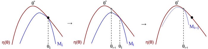
Let’s get into more details. We start with an initial policy guess. We find a lower bound M that approximate the expected reward η locally at the current guess. We locate the optimal point for M and use it as the next guess. We approximate a lower bound again and repeat the iteration. Eventually, our guess will converge to the optimal policy. To make this work, M should be easier to optimize than η. As a preview, M is a quadratic equation

but in the vector form:

It is a convex function and well studied on how to optimize it.
Why does the MM algorithm converge to the optimal policy? If M is a lower bound, it will never cross the red line η. But let hypothesis the expected reward for the new policy is lower in η. Then the blue line must cross η (the right side figure below) and contradict that it is a lower bound.
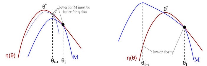
Since we have finite policies, as we keep the iteration, it will lead us to a local or a global optimal policy.
Now we find the magic we want.
By optimizing a lower bound function approximating η locally, it guarantees policy improvement every time and lead us to the optimal policy eventually.
Trust region
There are two major optimization methods: line search and trust region. Gradient descent is a line search. We determine the descending direction first and then take a step towards that direction.
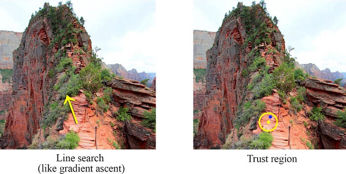
In the trust region, we determine the maximum step size that we want to explore and then we locate the optimal point within this trust region. Let’s start with an initial maximum step size δ as the radius of the trust region (the yellow circle).

m is our approximation to the original objective function f. Our objective now is finding the optimal point for m within the radius δ. We repeat the process iteratively until reaching the peak.

To control the learning speed better, we can be expanded or shrink δ in runtime according to the curvature of the surface. In the traditional trust region method, since we approximate the objective function f with m, one possibility is to shrink the trust region if m is a poor approximator of f at the optimal point. On the contrary, if the approximation is good, we expand it. But calculating f may not be simple in RL. Alternatively, we can shrink the region if the divergence of the new and current policy is getting large (or vice versa). For example, in order not to get overconfidence, we can shrink the trust region if the policy is changing too much.
Importance sampling
Importance sampling calculates the expected value of f(x) where x has a data distribution p.

In importance sampling, we offer the choice of not sampling the value of f(x) from p. Instead, we sample data from q and use the probability ratio between p and q to recalibrate the result.

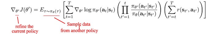
In PG, we use the current policy to compute the policy gradient.

So whenever the policy is changed, we collect new samples. Old samples are not reusable. So PG has poor sample efficiency. With importance sampling, our objective can be rewritten and we can use samples from an old policy to calculate the policy gradient.
But there is one caveat, the estimation using q,
has a variance of

If the P(x)/Q(x) ratio is high, the variance of the estimation may explode. So if two policies are very different from each other, the variance (a.k.a. error) can be very high. Therefore, we cannot use old samples for too long. We still need to resample trajectory pretty frequently using the current policy (say every 4 iterations).
Objective function using importance sampling
Let’s go into details of applying the importance sampling concept in PG. The equations in the Policy Gradient PG methods are:
We can reverse this derivative and define the objective function as (for illustration simplicity, γ is often set to 1):

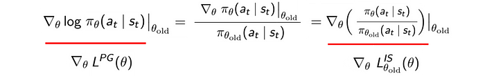
This can be expressed as importance sampling (IS) also:

As shown below, the derivatives for both objective functions are the same. i.e. they have the same optimal solution.
The presence of two policies in the optimization objective presents us with a formal way to restrict the policy change. This is a key foundation of many advance Policy Gradient methods. Also, it can produce a way for us to evaluate possible policies before we commit the change.
Now, we finish the three basic concepts we need for our discussion and ready for the last part for TRPO.
For those that what to look into the articles in this Deep Reinforcement Learning Series.
