Self-driving car: Path planning to maneuver the traffic.
Path planning is about finding a safe, comfortable and efficient path to maneuver around the traffic. The following video demonstrates the idea with green dots being our calculated trajectory.
This is part of a 5-series self-driving article. Other topics include
- Self-driving perception: Sensor fusion with Kalman Filter.
- Self-driving perception: Extended Kalman Filter and Unscented Kalman Filter.
- Self-driving localization: Localization with Particle Filter.
- Self-driving control: Control with Model Predictive Control & PID.
- Self-driving Path finding.
Workflow pipeline
First, let’s get an overview of the workflow.
Perception: We perceive what is around us. Through sensor fusion, we integrate sensor readings to construct a precise picture of the position and the velocity of our surrounding objects.

Prediction: We use the sensor information to predict the trajectories of our surrounding objects. So we avoid any collision.

Behavior planning: We look at different options and create a handful of proposals from our options. We eventually translate each proposal into a location.
Trajectory planning: For each potential target, we compute the corresponding trajectory.

Trajectory cost ranking: For each trajectory, we analyze its feasibility as well as the cost based on safety, comfort, and efficiency. We select the final trajectory with the highest score.

Control: Then we send the new trajectory to the car controller to control the actuators of the vehicle.

Here is the overview of a self-driving car system:

Perception
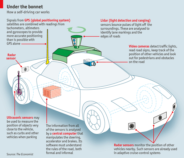
A self-driving car uses stereo cameras, LiDAR and Radar to perceive our surroundings. The video below shows the use of cameras to perceive objects around us so we know what actions are feasible and plan a path accordingly.
However, it is not easy to determine depth with stereo cameras. LiDAR sends out about 2000 pulses of near-infrared laser beam per second to reconstruct a 3-D world around us. RADAR, on the other hand, has longer range than LiDAR but lower resolution. It also has the capability to measure velocity.
Using sensor fusion, we reconstruct a consolidated and more accurate picture of the location and the velocity of objects.
Prediction
However, just knowing the location or velocity of objects around us is not good enough. We also make predictions on our trajectory and others to avoid collisions. If the trajectory of the self-driving car gets dangerously close to any other trajectories, we should increase the trajectory cost dramatically so we will not pick this choice.
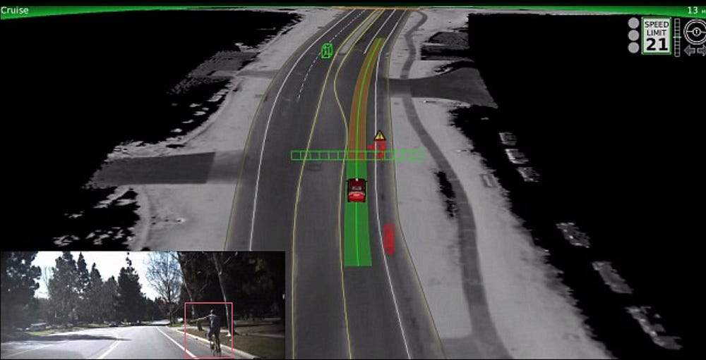
In an urban environment, we need to track far more objects including pedestrians, bikers, carts, scooters, etc… Sometimes, the hand signal of bikers and the posture of pedestrians are critical information in determining their intentions. The TED talk below lays down some fine details in such process.
Mode based or deep learning based trajectory prediction
To predict trajectories, we can use a model-based method or a deep learning method.

For a model-based method, we start with the dynamic model of an object.
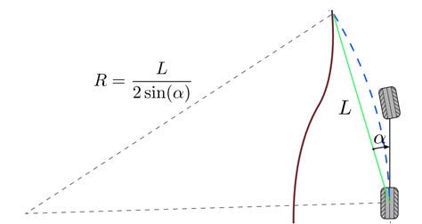
At each time-step, we monitor its motion predicted by its dynamic model, and estimate what is the likelihood of those possible trajectories.

Alternatively, we use deep learning to locate an object and to compute its trajectory or to classify its intention. For example, in the image below, we detect a biker is signaling a left turn.
Behavior planning
In conjunction with a map, a planned route to a destination and predictions, the behavior planner make suggestions on how to maneuver a car.
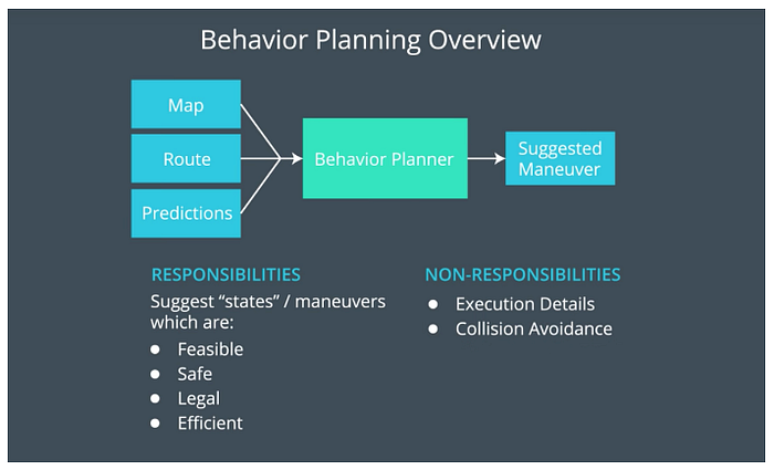
We are provided with many options:
- Lane: keep the same lane, switch lane(s) to the left/right, pass the vehicle ahead or just preparing lane change.
- Speed: keep the same speed, follow the vehicle ahead, slow down or accelerate to a target speed, or stop.
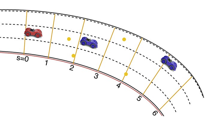
Start with different high-level objectives, like following the traffic, passing slow-moving cars, or speeding up to the speed limit. We look at different options on how to make it happens. For example, switch to the left lane and accelerate to 55 mph, or slow down to maintain a safe distance from the car in front. For each plan, we determine which lane to use and our target speed at the end of our evaluation. Then we calculate the location accordingly. Below, we come up with a list of locations (yellow dots) that we may want our car to be in say 2 seconds.

Trajectory planning
Once we have a list of candidate locations, we compute the trajectory for each proposal. But before that, we first take a look at the coordinate system.
Coordinate system
Localization and route planning use a global Cartesian system to define a location (x, y).
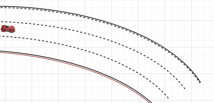
However, for trajectory planning, it will be easier to work on a coordinate system that following the curve of the roadway (Frenet frame). In our example below, we have 3 lanes. d=0 is the middle of the roadway. d=-1 means the right lane. s measures the distance from a specific point along the roadway. So instead of (x, y), our trajectory location is measured as (s, d) in the Frenet frame.
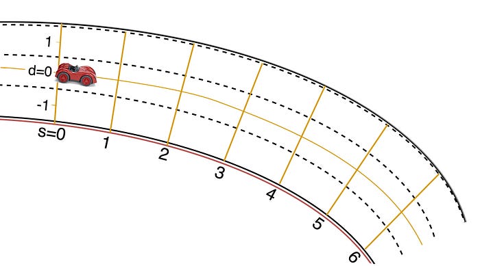
For display purpose, we warp the Frenet coordinate system as follows:

Conversion between the Cartesian and Frenet frame
We will use a map to convert coordinates between the global Cartesian and Frenet coordinate. However, the waypoints of the map may be farther apart than we want. For example, the map below has only 3 waypoints (pink). To interpolate points in between, we use these 3 points to fit a spline model, and use it to perform the transformation.

Now, let’s look into how trajectories are calculated.
Cubic spline model
During behavior planning, we propose different plans. We translate this into target locations that we want our car to be at a specific time. We use this target location and a few previous locations to build a cubic spline curve to model our trajectory. This spline model preserves the first, and second derivatives of our previous trajectories so we will have a smoother ride (no sudden jump in the velocity and acceleration). Later, we use the spline model to calculate where the car should be for every 0.02 second in the next second. Then, this information is transferred to the controller to control the actuators of the vehicle.

JMT (Jerk Minimized trajectory)
Alternatively, we can create a trajectory to minimize jerk which we want to minimize sudden accelerations. Mathematically, we define s as a polynomial function of time t. To minimize jerk, we want to find an optimal trajectory that minimizes the accumulated magnitude of the acceleration change, i.e. not too many sudden changes of acceleration |a’(t)|:

To accomplish this, we constraint our polynomial s(t) into a rank of 5. Intuitively, the high ranking of a polynomial allows sudden movement. For example, a rank 9 polynomial function below allows sharp turns.

To simplify the computation, we reset the time to 0 when we compute a new trajectory. We know our initial state (location, velocity, acceleration) from our car system.

and the behavior planning provides us the target state:


Now, we want to find the 6 coefficients in our trajectory model:

At time=0,

So the first 3 coefficients can be found from our initial state. We repeat if for our target state:

Now, we have 3 more equations so we can solve the remaining 3 coefficients. We will repeat the same process in finding the polynomial in the d direction.

Example

Ideally, during behavior planning, we want no more acceleration or lane change by the end of our planned trajectory. So for both initial or target state, they should be:

Also, our plan wants the car to reach a specific speed sometimes. (reaching the speed limit or match the speed of the car in front)

Here is our summary:
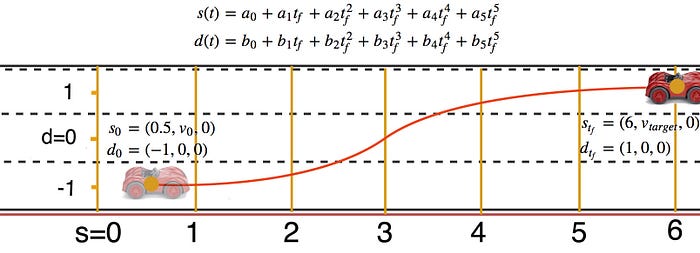
However, in low speed, we cannot calculate s and d independently (paper). In our example, we just make d=constant to get around the problem in low speed. (i.e. we don’t change lane at low speed)
Trajectory cost ranking
Trajectories are ranked using a cost function. Depending on our defined policy, it includes factors like
- the boundary conditions, the desired target of the state parameters, and
- the corresponding frequency and the magnitude of changes.
For example, the maximum acceleration is limited by the maximum torque of a car. So it is not feasible for a trajectory requiring an acceleration higher than what it can do. To avoid a collision, we compare all projected trajectories. We increase the cost dramatically when the car distance falls below a safety zone. For efficiency, we want to drive as close to the legal speed limit as possible.
We will also include more state parameters in the cost calculation. For instance, we will add steering angle and steering speed to avoid rollover. However, we do not count those factors equally. For feasibility and safety, their weights are extremely high. This makes sure we do not take an infeasible or risky move. Some other weights are tunable. So for less critical factors involving comfort and efficient, we conduct experiments to strike a good balance between a smoother ride or a more aggressive driving for the optimal speed.

After calculating the cost of all trajectories, we select one with the lowest cost as our final decision.
Produce new path
Now an optimal trajectory is selected. In our example, we compute the next 50 locations (0.02 second apart) using the mathematical model we build. i.e. 1 second of trajectory points.

We convert it back to the global coordinate. This x, y coordinate will be used by the car controller to maneuver the car and for localization purpose. However, usually we do not wait until the whole trajectory to complete for the next trajectory. Often, once we have a new set of measurement, we may re-compute a new trajectory.
Bonus
For fun, this is another way to send your Tesla to Mars if your path planning is off.
More thoughts
This article describes a bear bone framework for the path planning. This framework will be expanded and modified to meet the real-life challenge in particular for the urban driving.
Throughout the article, we frequent mention sensor fusion and control. For those interested in the technical aspect, here are a few more articles that you can read.
For readers that want more details in the trajectory optimization, this paper can be a good start.
