Speech Recognition — ASR Decoding

With the acoustic, pronunciation lexicon and language model built and discussed in the previous article, we are ready to decode (transcript) the audio clips into words. Conceptually, our objective is to search for the most likely sequence of words according to these models.
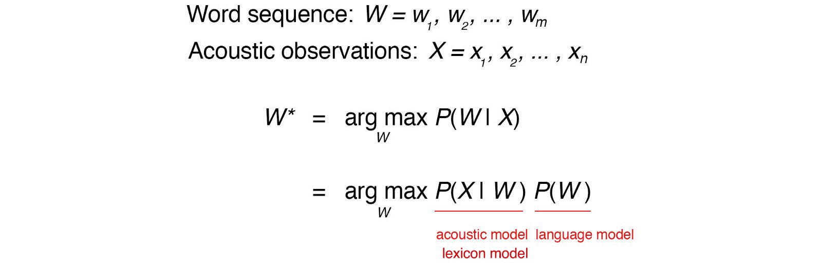
However, searching for all the possible sequences sounds astonishingly inefficient. Fortunately, in the HMM article, we can use the Viterbi algorithm to find the optimal path in polynomial time.

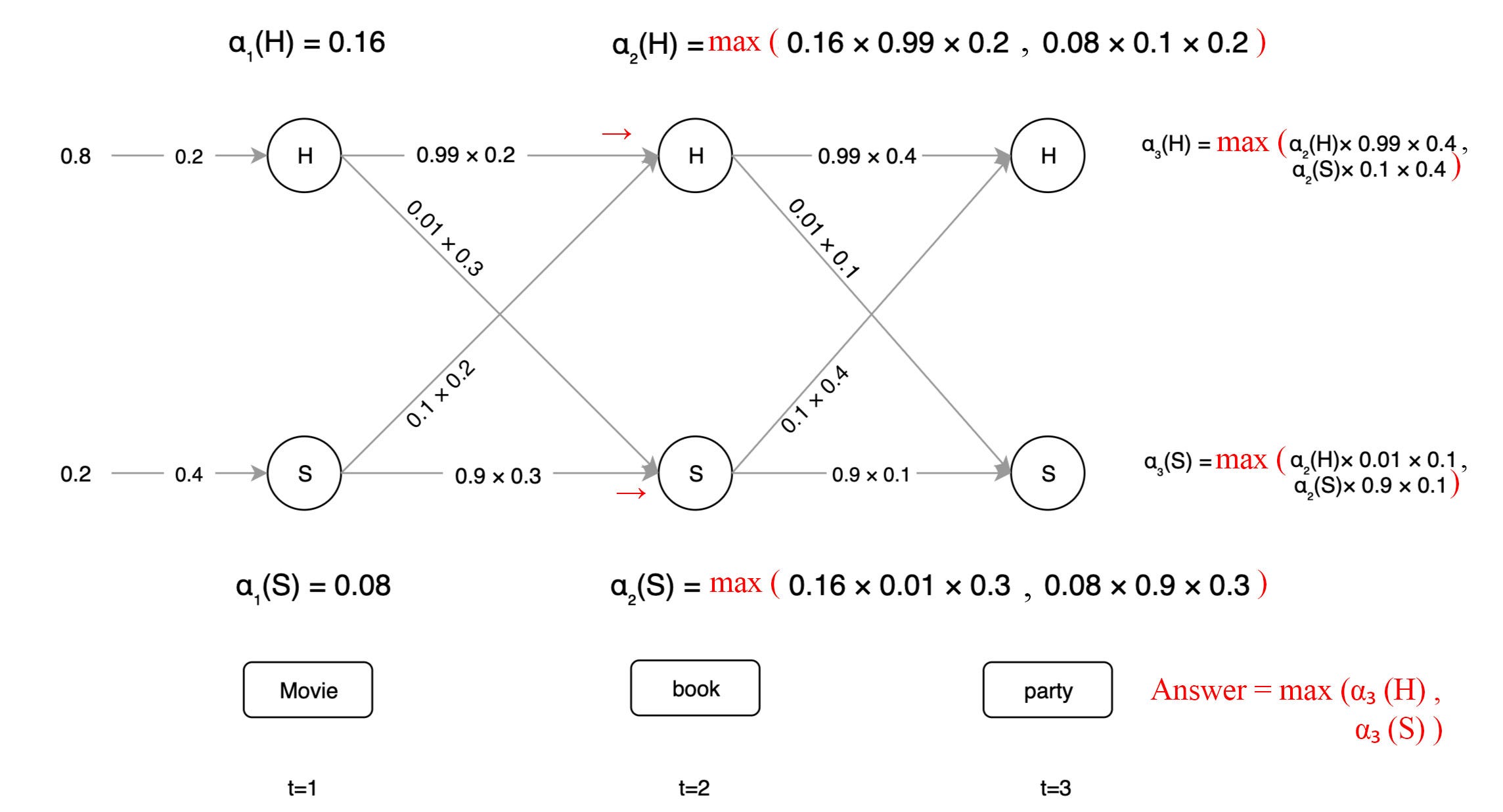
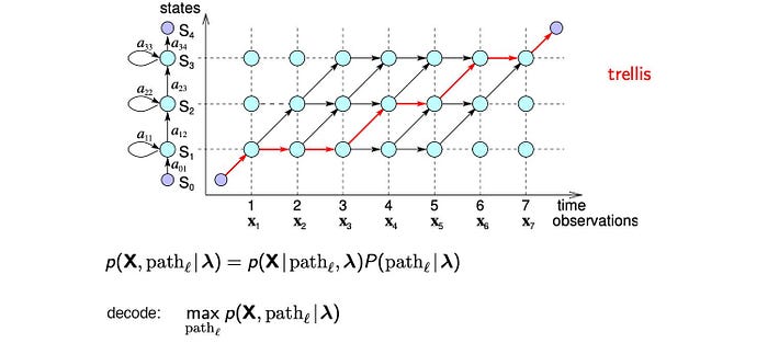
Recall the recursive equation used in the Viterbi algorithm.

We work from the left to the right in finding the most likely path in answering our observed audio features.
Here, comes the hard part in ASR.
Large Vocabulary Continuous Speech Recognition LVCSR
A complex ASR involves a large vocabulary size. The speech is continuous with word boundaries harder to know. Other challenges include:
- Huge searching space that exact decoding may not be possible.
- Long-span language model, like the trigrams, increases the search space significantly.
- Handling cross-word triphone — the acoustic depends on the first phone in the next word.
Many techniques learned from small vocabulary speech recognition are applicable in LVCSR. But let’s discuss some difference here:
- Alignment: the time information regarding the start and end of phones are less explicit in LVCSR.
- The HMM model for small vocabulary recognizer can be less complex with fewer states. Because of fewer states, it can afford to have one acoustic model (GMM) per state.
- LVCSR requires context-dependent modeling (triphones).
- The triphone concept increases the HMM states significantly. It requires triphones to share an acoustic model if they sound similar.
- LVCSR needs to train a decision tree to cluster triphones to share acoustic models.
While the Viterbi Algorithm is good for short commands with a small vocabulary, finding an exact solution for LVCSR, with the Viterbi Algorithm alone, seems infeasible. LVCSR requires more extensive combinations of methods. In particular, the search space will be pruned constantly to explore promising sequences only.
Weighted Finite-state transducer (WFST)
Kaldi is one popular toolkit for speech recognition research. The decoder is based on WFST. An HMM model is a state machine. For example, the HMM triphone model can be represented in the state machine below. It identifies the possible sequence of HMM states related to a phone.

Again, the pronunciation lexicon can be represented with a state machine. The following is the graph on how the word “data” is pronounced which includes possible variants in the pronunciation. For example, the phoneme /d/ can be followed by /ey/ or /ae/. The arc also indicates the corresponding probability. For example, for the word “data”, there is a 0.3 chance to pronounce the third phoneme with /t/ or 0.7 chance with /dx/.

Finally, the language model can be defined by a state machine too. The following is a bigram model in which the current word depends on the last word only.
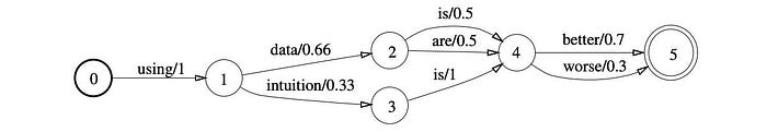
For example, the sequence “using data is better” will be more likely than “using intuition is worse” in the language model above.
This concept can be repurposed to match a sequence of labels to another output.
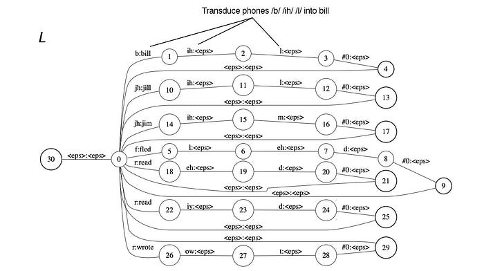
If the state machine matches the phoneme sequence /b/ /ih/ /l/, it will output the word “bill” followed by empty outputs (<eps>) that we will ignore. This state machine is called the Weighted Finite-State Transducer WFST. It maps a sequence of input to output.

Consider the four WFST transducers below.
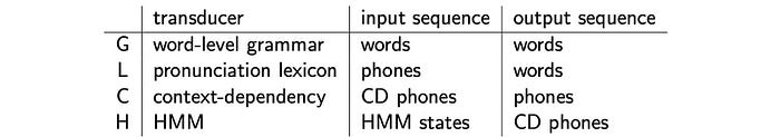
An HMM transducer maps HMM states to context-dependent (CD) phones. A context-dependency transducer maps CD phones to context-independent (CI) phones so we can map them to words. The first diagram below is a phone sequence of a word. The second diagram is the corresponding transducer from CI phones to CD phones. In ASR, we apply the inverse of the second diagram to make such a conversion.

The final two transducers convert phones to words and then to grammatically-sound sentences. We can combine these transducers to form one large decoding graph (searching graph). In speech recognition, we compose the transducer together (H ◦ C ◦ L ◦ G) to form a single decoding graph to covert HMM states to words. This process results in a huge HMM. In theory, we can use it with the Viterbi decoding to find the most likely sequence of words.
In reality, this involves a whole lot of works and simplifications. We need to optimize this huge graph for faster decoding. We apply determinization (det) to make it easier to search deterministically and minimization (min) to reduce the number of redundancy in states and transitions.

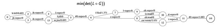
Here is a simple example of composing the lexicon model L with the language model G. It matches the phones /b/ /ih/ /l/ /#0//f/ /l/ /eh/ /d/ /#0/ into “Bill fled” or /jh/ /ih/ /m/ /#0/ /r/ /eh/ /d/ /#0/ into “Jim read”. Of course, the composition of the real transducers will be much larger and complex.
But the graph remains too large to search in practice for LVCSR. We apply beam-pruning with the Viterbi decoding (discussed later in this article). This trims away less promising searches to improve efficiency. This requires a lot of explanation and we will dedicate a full article on it. For the remaining of the article, we will focus on more advanced topics in improving the accuracy, or the decoding speed.
Evaluation
But first, let’s talk about ways to evaluate the accuracy of ASR?
WER (Word error rate)
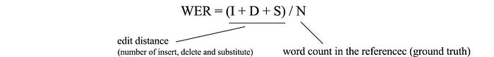
The most popular metric in ASR is WER. Consider a corpse with N words, WER (Word error rate) is the ratio on how many insertions, deletions, and substitutions (a.k.a. edit distance) are needed to convert our predictions to the ground truth.
Here is an example in calculating WER.

Perplexity
Perplexity is defined as:

In our example, we first compute P(W) using a bigram model using the occurrence count.

Then, we normalize the probability with the number of words using the geometric mean. The perplexity is:

We can understand the perplexity through entropy. Perplexity is the exponential of entropy H.

We use perplexity to measure how well a probability distribution in making predictions. For a good LVCSR and language model, the prediction should have low entropy and perplexity.
Intuitively, we can view perplexity being the average number of choices a random variable has. In a language model, perplexity is a measure of on average how many probable words can follow a sequence of words. For a good language model, the choices should be small. If any word is equally likely, the perplexity will be high and equals the number of words in the vocabulary.
Objective function
The acoustic model P(X|W) is estimated by multiplying individual probabilities P(xᵢ | pᵢ) together.

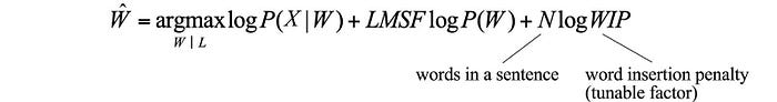
However, this independence assumption underestimates the real probability for likely phone sequences. The whole is greater than the sum of its parts in such a scenario, i.e. P(X|W) > ∏ P(xᵢ | pᵢ). Previously, we introduce triphone and dynamic features (delta and double delta) to take phone context into account. But its scope is less extensive in comparison to the language model. A bigram can cover half a second of audio data while a triphone may only relate to 75ms of the audio. Therefore, P(X|W) is relatively underestimated because of less context information is utilized. To counter the underestimation, we add a tunable language model scaling factor (LMSF) to recalibrate the relative impact of the acoustic model and the language model in the objective. Because log P(W) is negative, our LMSF factor should give the language cost a higher multiplier (say 5 to 15) to boost the acoustic score.
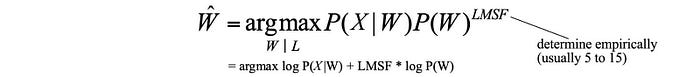
But a higher value of LMSF makes our decoded transcript to have higher deletion mistakes since a higher value penalizes the word transition higher. To counter this negative impact, we introduce another tunable parameter to balance between insertion and deletion error. In addition, we will use the log-likelihood for the objective function to improve numerical stability. So the final objective function is:
All these parameters will be tunned as hyperparameters in the process.
Beam Search
The curse of exponential search space haunts ML. One solution is pruning the search tree to limit the size of the search space. During searching, we prune branches when the cost or the probability reaches some predefined threshold. Or we can keep the number of branches to a certain size.

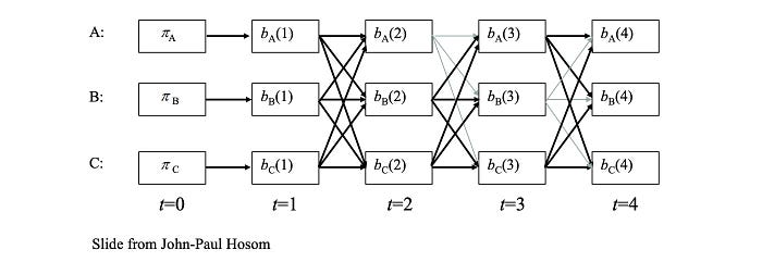
Viterbi Beam Search
Such kind of beam search concept is popular in many deep learning or machine learning ML problems. For ASR, we can apply it to the Viterbi algorithm to limit the number of searches for the maximum path. For example, we will not consider the path in gray below to limit the size of the search space.
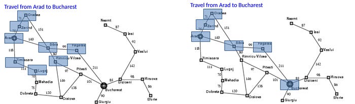
A* Search (Best-first search)
Beam search is a breath-first search. We explore all the next arcs from all active search path. But we eliminate those that show less promising. A* Search is a depth-first search. It searches a branch (an arc) with the highest probability or the lowest cost first. We keep expanding the search until we reach the final state. Here is an example of demonstrating the breath-first search (left) and the depth-first search (right) in finding the traveling path from Arad to Bucharest.
Multipass Search
Many ML problems struggle between scalability and capability. In ASR, we can use a faster recognizer to decode possible candidates. Then, we switch to a sophisticated model to select the final answer. For example, a long-span language model increases complexity dramatically while improving accuracy. So we may use a bigram model for the first pass and switches to 6-gram model for the second pass. Or in the second pass, we apply natural language parsing.
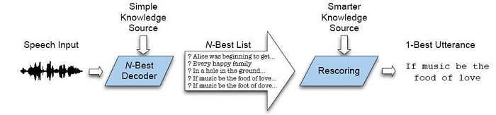
There are many ways to representing candidates for further selection later.
- N-best list — a list of N candidates.
- Word lattice.
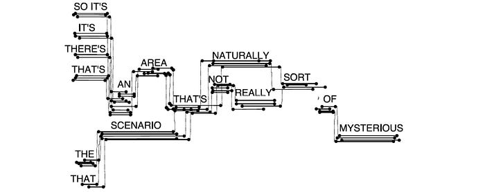
- Word graph in the form of Finite State Acceptor (a concept similar to WFST but with no output labels). A word lattice above preserves when a word may start and end. A word graph does not have this information for the words. However, a word graph or a word lattice can be referenced as a lattice sometimes. So just be careful in the terms sometimes.

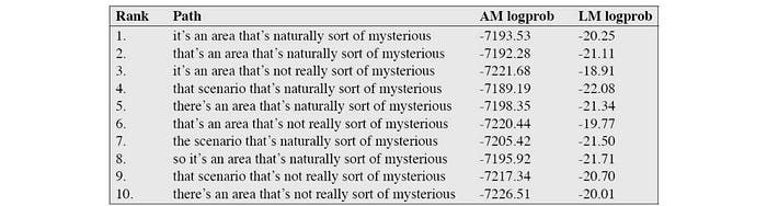
To find the best N-list in an HMM model, we may need to modify the Viterbi algorithm to keep track of the promising paths instead of the best path. Alternatively, we can compute the forward probability in the HMM model and perform N-list search using these probabilities.

But the best N-path is different from the best N-list. For the former one, we may end up with lists with words that are almost the same. We may modify the Viterbi algorithm to work with paths with the granularity of words instead of states. In a nutshell, we are not tracking information on the N-best sequence of states for each node, we are tracking the N-best sequence of words. At each node, we preserve the total probability for each of k (k = 3 to 6) previous words (possibilities). When a node may reach the end of a word, we sum over all possible paths for the word and consolidate the calculation as a single case. We record the score and name for each previous word. So for these nodes, we have a record of different word sequences and their corresponding score. But we just pass on the best word sequence for the next iteration. When the end of utterance is reached, we follow the back pointers for the best word sequence. But during the backtracing, we also put the alternative previous word ending on a queue. To find the next best, we pop the next best from the queue. There are many fine details but we will let the readers doing their own research.
Next
We have put off the discussion of one popular decoder. It is time to get to WFST in more details.
Otherwise, you can go ahead to see how ASR is trained.
Credit & reference
Speech Recognition with Weighted Finite-state Transducers
Weighted Finite-State Transducers in Speech Recognition
Speech recognition — a practical guide
