Speech Recognition — ASR Model Training

Now, we come to the last part of the puzzle in training an ASR. In this article, we will dig deeper to learn how to train the models for ASR. But, when ideas are moving from research to deployment, expect the training to be insanely complex. To push the limits, many heuristic methods, including trial and errors, are used. It may not be an overstatement to say the training is one big hack. The resource needed to train a commercial LVCSR is enormous. The details are tedious. Many domain knowledge, as simple as the length of the training, is kept as trade secrets. In discussing the ASR training, we will focus on the key aspects rather than on the engineering bolts and nuts. But even for that, there are a lot of grounds to cover. Since this is one of the last major topics for this series, let’s do a quick recap of what we learned first.
Recap (optional)
Our ASR objective is finding the most likely word sequence W* according to the acoustic observations, the acoustic, the pronunciation lexicon and the language model.

The first step is to extract features from audio frames using a sliding window.

Each audio frame will contain say 39 MFCC features. This forms a sequence of our observations X (frames: x₁, x₂, x₃,…, xᵢ , …).
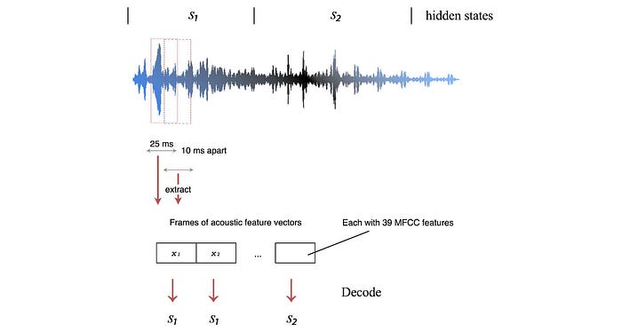
The extracted features include information of the formants in identifying a phone as well as their first-order and second-order derivative in understanding their context.

Our task is to reverse engineering the internal sequence of states (s₁, s₂, s₃, …) from the observed feature vectors X.

The key idea is finding a state sequence (a path) that maximizes the likelihood of the observations.
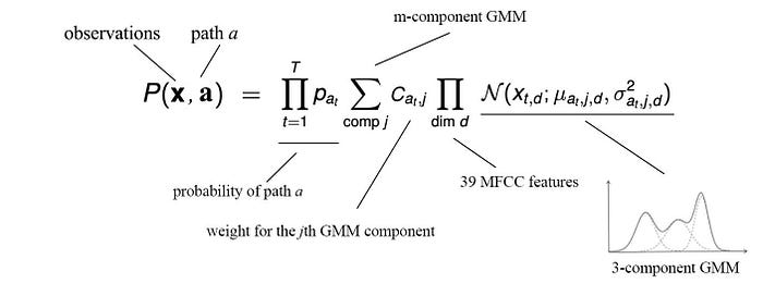
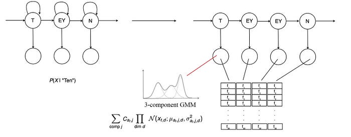
The R.H.S. above contains the probability of a path and the likelihood of an observation given an internal state. Let’s look into the second part closer. Each word will be modeled by a pronunciation lexicon and an HMM. The self-looping of a state allows ASR to handle different duration of phones in utterances. The likelihood of an observation given a state will be modeled by an m-component GMM.
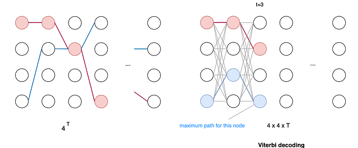
Searching for such sequence one-by-one, even with limited sequence length T, is hard. With a vocabulary size of k, the complexity is O(kᵀ) and grows exponentially with the number of audio frames.

Fortunately, Viterbi decoding can solve the problem recursively. For each time step, Viterbi decoding computes the maximum path for a node using results from the last time step. So we can search the exact maximum path in O(k²T).
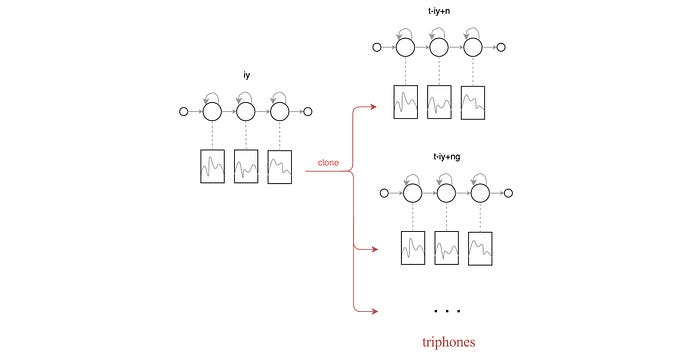
Nevertheless, to increase ASR accuracy, we need to label the phone with its context also. Unfortunately, this grows the internal states to 3 × 50³ states if we start with 3 × 50 internal phone states. To address that, some labels with similar articulation will share the same acoustic model (the GMM model). The diagram below demonstrates the journey from 3 states per context-independent phone to 3 states per triphone using GMM.

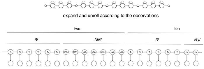
We can simplify our HMM topology drawing by writing the output (emission) in an arc. The following represents the word “two” that contains 2 phones /T/ and /UW/, each modeled by three states.

To handle silence, noises and filled pauses in a speech, we also introduce the SIL phone.

Once we build an HMM model for a word (the left diagram below), we can concatenate and loop them back to handle continuous speech. Now, we can use Viterbi decoding again with a new graph to handle continuous speech.

To improve the accuracy of ASR, we can compute the transition probabilities between words using a language model. In the model below, we simplify the language model into a bigram.

In a bigram (2-gram), the next word depends on the previous word only.

We can extend the language model into n-gram. The following is the state diagram and the transitions for the bigram and the trigram model respectively.
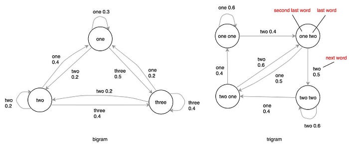
Here is the visualization with a trigram language model

In the end, we introduce the concept of Weighted Finite-State Transducer WFST to model the HMM triphone model, the pronunciation lexicon, and the language model respectively.

By introducing the four transducers below:

We manage to decode audio into a word sequence.

But to make this efficient, we will compose transducers together.

And optimize and pre-compile them for decoding.

The diagram below is the conceptual flow of an ASR in decoding.
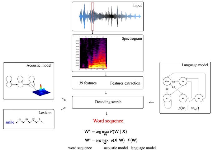
If you don’t have a single clue of this overview, you may need to read from the beginning of this series first. The description so far is for decoding. In training an ASR, we focus on learning the HMM model using features extracted by the training dataset. The lexicon models and the language models have been discussed before and not too hard to learn. So we will not elaborate further.
The key focus of the ASR training is on developing the acoustic model for the triphones (the context-dependent phones).

ASR
The ASR model for a single digit is pretty simple. The following is the HMM topology for the digit “six”.

We can connect the HMM models for all digits to form an ASR in recognizing digits.

Next, we ask how hard to train a Large Vocabulary Continuous Speech Recognizer (LVCSR). The following is the HMM in recognizing continuous speech. The topology is a simple concatenation of HMM models. The basic components are the same as a single word recognizer.

But, when we add a language model to LVCSR (right diagram), the graph can become crazily complex.

But thanks to the WFST, we can componentize them into separate models. The language model is modeled separately with a corpus using simple occurrence counting. Composing all the models together (H ◦ C ◦ L ◦ G ) is tedious but we will let the library like OpenFST to do the dirty works. But here are the few new challenges for LVCSR in training.
- Pronunciation is sensitive to neighbor phones (context) inside a word and between words.
- The alignment between HMM states and audio frames are harder for continuous speech.
- A large vocabulary triggers a lot of states to keep track of.
For accuracy, LVCSR needs a complex acoustic model and a far larger number of HMM states to model the problem. The first issue will be addressed by the GMM for now and the second issue will be addressed by triphones to take phone context into consideration. With the basic HMM topologies to be the same as a single word recognizer, many training concepts can be reused. But there are some important exceptions. First, the acoustic model for each HMM state is more complex. That introduces a major headache in training. As the complexity grows, it may get stuck in bad local optima. Like other complex ML models, we need a good strategy to learn it. Second, we need to perform alignment more frequently. Third, the potential number of acoustic models is so large that similar-sound HMM states need to share the same acoustic model. We will train a decision tree to cluster what triphones will share the same models. Next, we will discuss a few key concepts before detailing the training steps.
Training strategy
Rome is not built in one day. Training commercial quality ASR takes weeks using a cluster of machines. Training any complex Machine Learning (ML) and Deep Learning (DL) models take time and patience. We want the training to provide an optimal solution. ASR trains the model in stages (multiple passes). In many optimization problems, we solve the problems numerically with an initial guess. If the objective function is concave, we can guarantee the solution to be a global optimum.

If not, we will likely reach a local optimal instead.

In ASR, the presence of hidden states in HMM makes local optimal issues more problematic. But if the acoustic model is simple enough, the corresponding cost function may be much smoother and the global optimal is more dominant. i.e. it will not be hard to find. (Note: this is a general assumption or belief.)

But this model is biased. We need to do better and make it more complex. Since the HMM topology remains the same, if the next acoustic model is a superset of what we have trained, we can seed the new model with the old model parameters. This gives us a headstart for the next phase of training. More important, it may help us to stays away from nasty local optima. If we start with random guesses, we may be stuck in a terrible local optimum.
In ASR, we start the training with the more simple context-independent (CI) phone model. And each emission (output) in the HMM is first modeled with a single Gaussian (a 1-component GMM).

We initialize the mean and the variance of the Gaussian to be 0 and 1 respectively. Even with this naive guess, a reasonable model can be built using the training dataset. Getting close to the global optimum should not be hard for this model. Once the models are trained, we use them to seed the parameters of more complex GMM models. Say, we move from 1-component GMM to 2-component GMM and then double the components in each pass. We will do it gradually to make sure we do not jump the gun.

Once we build a context-independent CI model, we can switch from the CI training to a context-dependent (CD) training by cloning the CI GMM parameters to the new CD GMM model. Then, we start labeling HMM states with triphones. This strategy allows us to gradually build up more complex hidden states and acoustic models.
Forced alignment
The acoustic models are defined as P(x | HMM state) where x is the observed features in an audio frame.

Many training corpora are phonetic transcripted and the HMM topology for each phoneme is manually defined. In the design below, each phoneme is sub-divided into three HMM hidden states.

An HMM state can span over multiple frames. The self-looping structure models different durations of the HMM state in the utterance. This provides a flexible model to accommodate variants in speakers and speaking speed.
Forced alignment identifies the HMM state corresponding to an audio frame.

The transcript is time-aligned with phonemes. So we still have to further align the audio frames with the HMM states. We will do it programmatically.

In addition, for LVCSR, the phoneme alignment may not be perfect. Also, there may be silence or noise between phones. We need further alignment using the observed audio frames.
This alignment task finds the most likely HMM state sequence corresponding to the observations. This is not easy since we don’t know the HMM model parameters yet.
Forward-backward algorithm (FB)
Fortunately, we already learn one ML algorithm to solve this problem. That is the Forward-backward (FB) algorithm in HMM. Here is a quick recap. Using the HMM model, we apply the forward algorithm to learn the distribution α of the hidden states at time t given all the observations observed so far. We reverse the direction for the backward algorithm to find the distribution of the hidden states β at time t given the observations that we should see.

From the forward and backward probability α and β, we compute the state occupation probability (γ) and the transition (ξ) in maximizing the likelihood of the given observations. These values will be used to re-fine the HMM model. We keep iterate. γ and ξ estimation will be improved by aligning a better HMM model with the observed audio frames. Better γ and ξ produce a better HMM model.

The alignment implied by the FB will also be improved in each iteration.

By the end of the process, each audio frame in the corpus will be correlated to an HMM state.

We group them together to estimate the feature distribution for a given state P(x | HMM state) — the acoustic model. However, this explanation is not exactly correct. FB is an EM algorithm using a soft assignment. It computes the chance of an HMM state at time t with the observed audio features. The one described is a hard assignment that assigns an audio frame to one state only. FB uses soft assignment. If you want more details, you can find it here. But if you don’t know the difference, you can just move on and fake it as a hard assignment for easier understanding. In our context, you just need to know one important point. To compute the probability of being in a state at time t, FB sums over the probabilities for all possible paths reaching this state.
Viterbi training
Therefore, FB is computationally intense. It computes the forward and backward probability by summing over all possible paths. But if we switch to a hard assignment concept, we just need to know what is the most likely state. Then assign the audio frame to that specific state. For example, for the utterance below, we can relate o₄ with ahf and o₂ with ahm.

This process just needs to locate the most likely state sequence. For this purpose, we can use Viterbi decoding to find such sequence and skip computing the forward and backward probability.
Don’t treat Viterbi training the same as Viterbi decoding. Both FB and Viterbi training starts with some initial HMM model. In Viterbi training, we use the Viterbi decoding to find the most likely path. This links a hidden state to an audio frame.

We go through all the utterances to estimate all the corresponding hidden states.

Now instead of a hidden model, everything is visible and we can re-estimate the HMM model parameters. Then we reiterate the process again by finding the best sequence with the new HMM model. So while Viterbi decoding finds the best state sequence, both FB and Viterbi training are EM algorithms in optimizing the HMM model parameters and the acoustic models in alternating steps.
Viterbi training is less computational intense. So if you can get away with it, go for it. But in early training, the acoustic models are less mature. FB may be considered. In practice, speed and simplicity may dominate the training result. So give the Viterbi training a chance first. Indeed, many practitioners may suggest that. When the HMM models become more mature, the difference in the soft assignment and the hard assignment are not significant and will produce the same result. (In this article, we may mention the use of FB algorithm in training the model. Likely, Viterbi training can be used instead.)
Alignment improves acoustic models. Good acoustic models improve alignment. Therefore, throughout the training process, we perform alignment whenever we have significant improvement in the acoustic model. When the model becomes more accurate, we will use it to correct mistakes in the transcript and introduce silence phones also.
Key training steps
Before the training, we collect
- Utterances with transcripts.
- We define the pronunciation lexicon for each word.
- We define the HMM topology manually.
We may want to determine the size of the model like the number of components in GMM. And we may want to determine what questions may be available for the phonetic decision tree.
Here are the major training steps:
- According to the reference transcript, we form an initial HMM topology.

The bottom diagram is the HMM topology representing the utterance “He is new”. It is derived from the transcript from the dataset, the pronunciation lexicon, and the phone models.
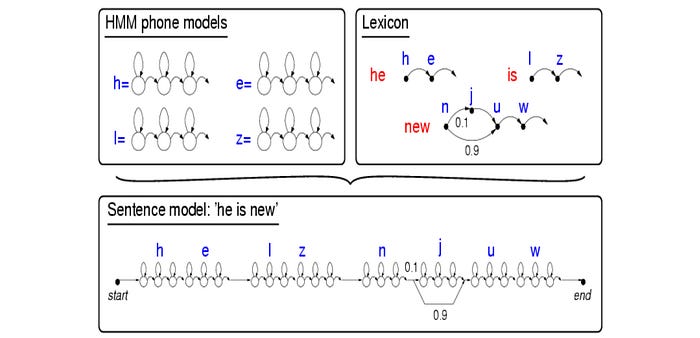
- Based on this topology, we build an acoustic model for each CI phones. To learn the alignment between the HMM phone state and the audio frame, we apply the forward-backward algorithm (FB).

- Then, the MFCC features in the aligned audio frame will be used as the training data in calculating the mean and the variance of the single Gaussian.

- Mixture splitting (details later): We start with this 1-component GMM (single Gaussian). We split each Gaussian into two and run many iterations of the FB. This realigns the audio frames with the HMM phone states. We continue the splitting, followed with many iterations of FB until reaching a target number of components in GMM. This acoustic model will get more complex gradually.
- Refine the reference transcript: In this phase, we select the pronunciation variant and spot the silence phones for the utterance. We perform further FB training to refine the transcript and the alignment.
- Use CI model and the refined transcript to realign CI phones with the training data. Then we build the phonetic decision tree (detail later).
- Seed (clone) CD models from the CI models:

- Retrain the CD model with the Forward-backward algorithm or Viterbi algorithm. We refine the acoustic GMM model and possibly with more mixture splitting.
As a reference, here is an ASR model example. This is the model for a 40K vocabulary in the North American Business News (NAB) task. (Typical English-speaking adults know about 42K words.)

(The number of Gaussian components can be much higher than the model above.)
If you have followed our speech recognition series, you should manage to understand most of the steps above.
GMM acoustic model
The major focus of ASR training is to develop an acoustic model. We start the acoustic model with a single Gaussian. Eventually, we want to develop a GMM for it.

To simplify the discussion, let’s say we extract one feature per audio frame only. With the forced alignment done, we collect the corresponding observed features in the training dataset to model the GMM model for the given phone state.

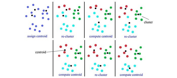
Say, we want to discover the components G1, G2, and G3 above, we can apply a k-mean clustering. The following is an example of the k-means clustering with k=3. But in this example, the extracted features are 2-dimensional instead of 1-dimensional.
Mixture Splitting
Instead of the k-means clustering, a popular approach is the mixture splitting. Starting from the single Gaussian, we split it into two with two new initial centroids separated from the original one by ε. We can choose ε to be proportional to the variance of the original Gaussian, like 0.2 × σ. However, we will disregard the split if there are not too many data points available for any split cluster.

So we split a Gaussian into two and run many iterations of the FB algorithm. Then we perform the split again. We repeat the iterations until reaching a target number of GMM components.
Phonetic Decision Tree
To improve ASR decoding accuracy, the training moves from CI (context-independent) phone models to CD (context-dependent) phone models. However, the combination of phones in creating context produces a huge number of phone states (triphones). The key idea of the Phonetic Decision Tree is allowing some triphones that sound similar to share the same GMM model (acoustic model). Before the training, we prepare a list of questions that we want to use for the decision stumps. We apply decision tree techniques to split data. We want to use fewest steps to cluster similar triphones together. So they can share the same GMM model. The following are some examples of such decision trees. The root node corresponding to a context-independent phone. The leave nodes are how we cluster context-dependent triphones in sharing the GMM models.

Again, we align phones with audio frames and build the decision tree according to the corresponding observed features and context.

Once such a decision tree is available, we are ready to switch from a context-independent training into a context-dependent training.
Refine transcript
With the word transcript, the pronunciation lexicon, the phone-level HMM, we compose an HMM in modeling the utterance.
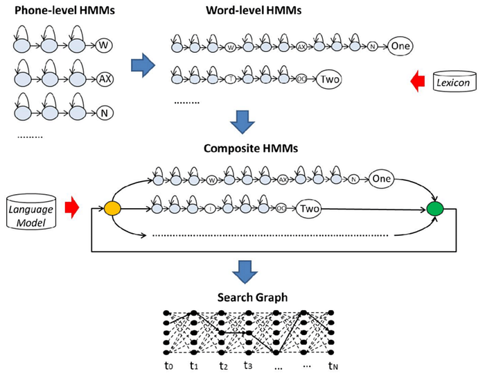
To reduce the complexity of the graph, we want the transcript to be as close to the utterance as possible with the fewest arc. In particular, we want to narrow down the exact pronunciation for words that have multiple pronunciations.

Noise
In addition, we want to refine our transcript to locate silence, noises and filled pauses in the speech. We introduce SIL as another phoneme in recognizing those sounds. SIL is always inserted at the start and end of an utterance. Without proper recognition of these silence sounds, it can break the recognizer. But these sounds are hard to model. There is a large variant of noises to cover sounds like breathing, laughing and background noise. We may use five HMM states instead of three to model them. We may introduce more SIL phonemes instead of one.
When the HMM model is reasonably good, we can perform the Viterbi algorithm to narrow down the silence phones and the exact pronunciation of words.

For later passes, include the generation of the phonetic decision tree and the CD phone model, we will use this refined transcript instead.
Here are the major steps in ASR training. But be aware, there any many other options and variants. Next, we take another look in alignment.
Alignment (Optional)
Alignment matches a transcript to a recording. However, some transcripts, like TV captions, may not match the audio exactly. For example, a transcript may skip or add words. If these audios are used for speech recognition training, we may need to prescreen them first and choose those utterances that have a good match with the transcript. This is called lightly supervised training.
First, we can interpolate a new language model based on the language model derived from the transcript and a regular language model learned from a corpus.

Then, we decode the training data with the existing acoustic model and the new language mode. This creates a more reliable transcript and alignment. For training, we choose utterances that match well between the captions and the decoded output.
Instead of building a distribution with the language model, we can build a new WFST language model derived from the transcript and use it to decode the audio. The G transducer below is called a factor transducer. It allows any substring of the original transcript to be detected.

And this is its deterministic version.

We can modify it again to allow words to be deleted from the transcript.

And this is its deterministic version.
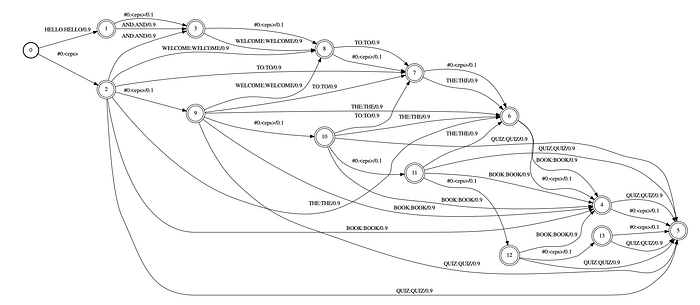
First, we can decode the audio with the factor transducer. We align the output with the original transcript and resegment the data. We then later decode it again with the second transducer above to allow words to be skipped in the audio. After it is done, we can compare the decoded words and the transcript to see whether we should accept the utterance for the training purpose. For more details, please refer to this paper.
Speaker adaptation
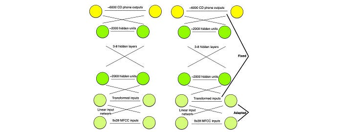
We can also train a model for speaker adaptation. In the deep network model below, we add layers to be trained to adapt to a specific speaker. This concept is very similar to the transfer learning in DL.
Next
Now, we have all the background information on training ASR. Kaldi is a popular toolkit for researchers in speech recognition. It is time to demonstrate how to train ASR with some solid examples.
