Speech Recognition — Deep Speech, CTC, Listen, Attend, and Spell

17 min readOct 13, 2019

Deep Learning (DL) changes many Machine Learning (ML) fields that heavily depend on domain knowledge. Decades of research in modeling this domain knowledge can be replaced with DL models with higher accuracy and less manual labor. In this article, we will focus on applying DL in speech recognition. But it is illusional to conclude ML will not play major roles to move us forward. Many complex AI systems, including the AlphaGo, apply many ML techniques. Speech recognition is no exception.

What is supervised deep learning?

Build a complex function estimator to make predictions.

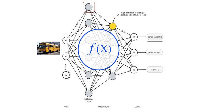
X is the input features. From this perspective, whenever we need a complex mapping between an input and an output, we can apply DL. Let’s recap the typical ASR approach (Automatic Speech Recognizer) in ML.

It involves a language model (say a bigram model)

, and an acoustic model likes

In the language model, the input is the previous word(s) and the output is the distribution for the next word. For the acoustic model, the input is the HMM state and the output is the audio feature distribution. We can model the distribution p(y | x) as f(x) using a deep network f.

But the acoustic model discussed before is a generative model p(x|s).

To adopt the same design, we compute p(x|s) from p(s|x) using the Bayes’ Theorem. The evidence p(x) is invariant of the word sequence. Therefore, it can be ignored in the optimization.

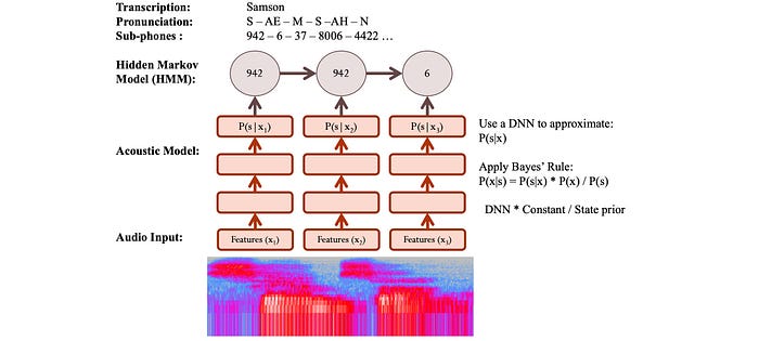
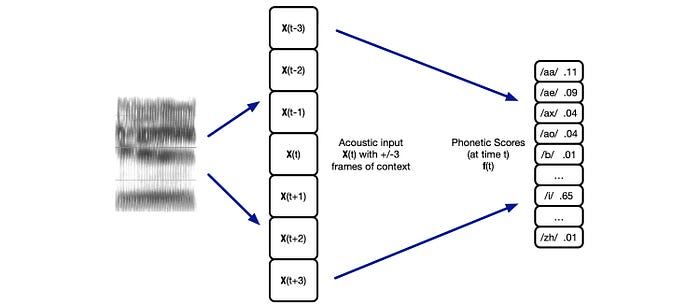
So given the features in an audio frame, we can use a deep network to predict p(s|x) and apply Bayes’ Theorem to estimate p(x|s) ∝ p(s|x) / p(s). In addition, we can include the neighbor frames as input. This creates a better phone context for better predictions.

Feature Extraction

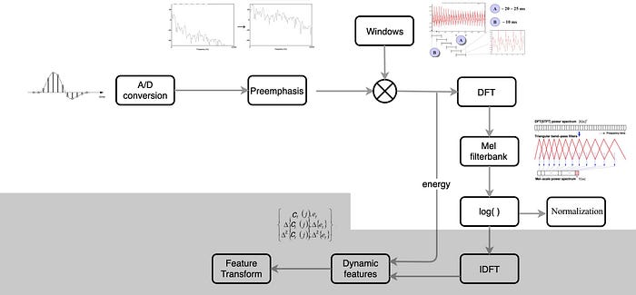
In ML speech recognition, we extract MFCC or PLP features from the audio frames. It includes steps like an inverse discrete Fourier transform (IDFT) to make features less correlated with each other. Also, we only take the lower 12 coefficients. In general, ML is more stingy in feature selection.

DL is good at untangling data and finding correlations. Therefore, it requires no or less pre-processing. It can handle a much larger number of input features and there is no particular need to un-correlate them first. We just need to design a more complex model and lets it learned from the data. In ASR with DL, we skip the last few steps including the IDFT. We simply take the Mel filter bank, apply the log and normalize it with the speaker or corpus’ mean and variance.

The next question we need to ask is what deep networks should we use. There are three major deep network categories.

Fully connected network (FC)

We can use the features from the Mel filter bank as input to an FC network. Some ASR FC models contain 3–8 hidden layers with 2048 hidden units in each layer. This model can predict the distribution of the context-dependent states (say 9304 CD triphones) from the audio frames. The following is an early comparison between a GMM-HMM ASR with a DNN-HMM (deep network). Lower values demonstrate better results.

CNN/TDNN

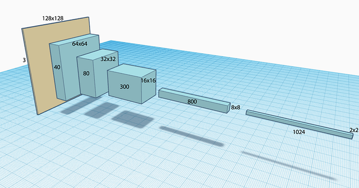
FC networks are computationally intense. It requires a lot of model parameters even for reasonable feature size. CNN takes advantage of locality and discovers local information hierarchically. CNN is more efficient if the information has a strong spatial relationship. It allows deeper layers and creates a more complex function.

Audio speech is time-sequence data. Instead of applying a 2D convolution filter, we use a 1-D filter to extract features across multiple frames in time. This is the Time-delay neural networks (TDNN). In the TDNN on the left below, the yellow box takes input from 5 nodes in the previous layers with each node containing 700 features.

This article assumes you have basic background in deep learning. So we will not explain many DL concepts in detail. Again, here are some ASR performance comparisons between the fully connected network and TDNN.

RNN (LSTM & GRU)

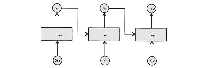
Solving a temporal problem with a spatial concept may not be ideal. Alternatively, we can use a deep network designed for time-sequence data. The following is the RNN. Each cell contains a cell state c and outputs h. The cell state is determined by the current input and the previous states including the previous cell state and the previous output.

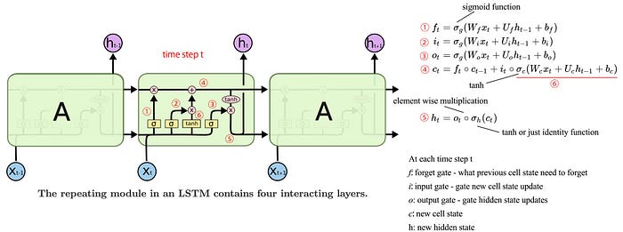
Below is the diagram for the LSTM (probably you would not understand the diagram until you are familiar with LSTM). It composes of the forget gate f, and the input gate i. f controls what information in the previous cell state will be forgotten. i controls what information in the current input and the previous output will be used to update the current cell state.

We can also stack the RNN cells to make the model more complex. Another possibility is bidirectional RNN. We have a forward pass and a backward pass with results combined later. For example, we add the result together followed by an FC layer.

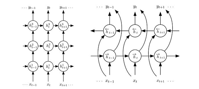
We can even combine both concepts together.

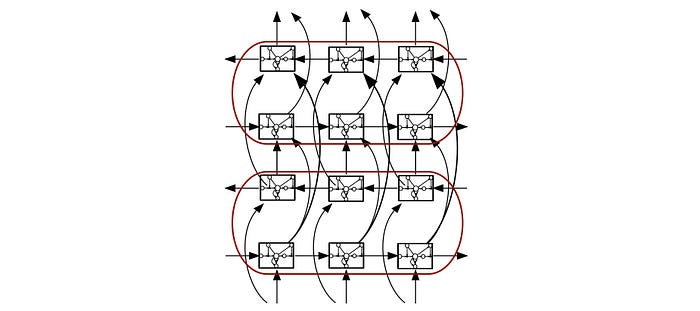
Here is an example of applying the concept above in classifying CD states.

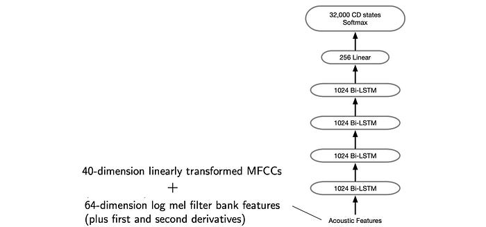
The following is the testing result for different models.

But so far we have only taken incremental approaches, like DNN Hybrid Acoustic Models, to integrate DL into the HMM models. Can we design a new approach from scratch?

Connectionist temporal classification (CTC)

ASR decoding is mainly composed of two major steps: the mapping and the searching.

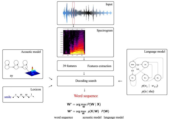
In the mapping, we map the acoustic information of an audio frame to a triphone state. This is the alignment process. This is a many-to-one mapping. It maps multiple audio frames to the same triphone state.

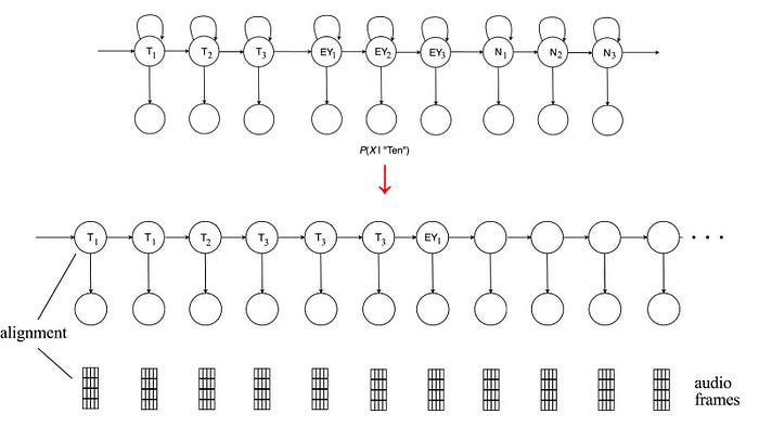
The alignment maps acoustic information to a phone. Then, we search for the phone sequence for the optimal word sequence. However, we need to account for multiple paths that produce the same results. This makes things complicated and requires us to use complex algorithms, like forward-backward (FB) or Viterbi algorithm.

DL learning is good at mapping. It opens the door for an alignment-free one-to-one mapping which maps an audio frame to a relatively high-level component. Then, we can search for it. This gives us a head start and bypasses the complicated alignment process. That is the core concept of CTC. While in early research, the deep network works with phonemes, now the deep network works with character sequences. This frees us further from the pronunciation lexicon and the phonetic decision tree.

The deep network generates a probability distribution for all characters. We don’t greedily pick the most likely character in each time step. There are multiple paths that represent the same word (details later). We need to sum over them to find the optimal paths.

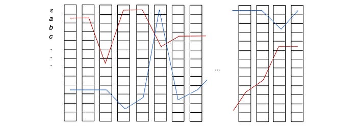
Since people pause in speech, within or between words, we introduce empty tokens <b> (or written as ε) to model such behavior. Other characters like ? and ! are also introduced. The following diagram indicates how we use bi-direction RNN to score characters for each observed audio frame. Then we apply softmax to create the probability distribution for characters in each time step.

CTC Compression Rule

Previously, we said multiple paths may produce the same word. Given the path “aaapεppllεe”, what is the word that it represents? For that, we apply the CTC compression rule. Any repeated characters will be merged into one. Then, we remove ε for the final word.

As noted in this example, to output the word apple, the deep network needs to predict a ε between the two pp in apple. Therefore, ε also serves the purpose of separating repeated characters in a word. Here are the valid and invalid predictions for the word “cat”.

The alignment-free concept in CTC actually pushes the complexity from mapping to searching. But by outputting character distributions and get rid of lexicon and decision trees, the search may not be that bad.

CTC Loss

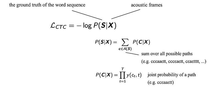
To find the most likely word sequence, we search for different path combinations. We need to sum over all paths that generate the same word sequence. For example, to find the probability for the word “hello”, we sum over all the corresponding paths like “heεllεlloo”, “hhellεεlεo”, “εeεllεεloo” etc.

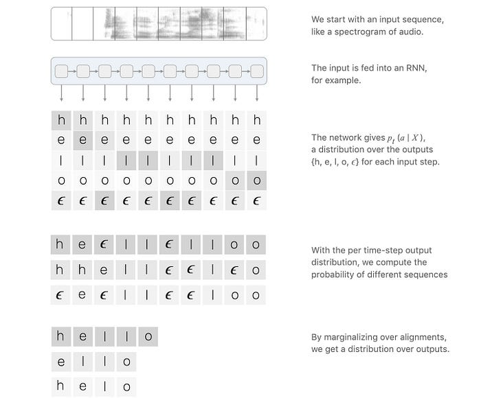
Here is the corresponding CTC loss function:

Dynamic Programming

In reality, CTC delays the complexity of the algorithm from the mapping to the searching. In CTC, we sum over all paths that produce the same word sequence. Then, we find the sequence with the highest probability. To calculate the probability of a word sequence efficiently, we apply the same principle in FB or Viterbi algorithm by restating the problem as a recursive problem and solve it with dynamic programming.

Dynamic Programming Details (Optional)

(Credit: the diagrams in this section are originated or modified from this source.)

In FB, we compute the forward probability α. We will do something similar here. The following diagram demonstrates the possible paths that can be observed as the word “ab” during the length of the observed utterance (say the length is 6 timesteps). The starting state is either “a” or “ε” and we will either land on “b” or “ε” at timestep 6.

Let's expand the decoded word say “ab” to “εaεbε” with “ε” added. We will call this expanded sequence Z. This is the vertical axis in our transition diagram. Let’s focus on the orange node below which recognize “εa” in Z already. For the next time step, there are three possible transitions. We can

stay with the same character for the next time step to the pink node,
transit to the next character ε in Z — the green node, or
skip the next character ε and transit to the purple node.

But skipping the next character in Z is not always a valid choice for certain patterns in Z. For case 1, if we have a pattern of “aεa” or “εaε” with “ε” or “a” be the next character respectively, we cannot skip it. We will reconstruct “a” and “” instead of “aa” and “a” after the CTC compression. Here is an example of “εbε” in demonstrating the issue. The cross-out transition below is invalid to produce “ab”.

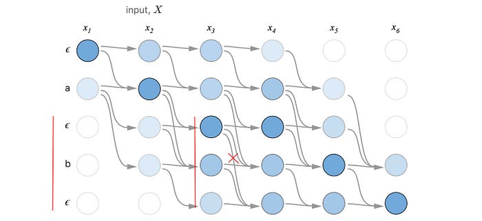
Let’s consider another case, i.e. case 2. If we skip the middle character of “aεb”, we can still reconstruct “ab”.

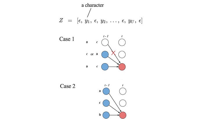
We can generalize this solution for any Z. Let’s α(s, t) be the CTC probability where we have realized the character 1 to s in Z at time t.

We can express α(s, t) in terms of the previous α recursively depends on the pattern in Z.

In short, we can consolidate paths that generate the same character sequence together. So we don’t need to handle them separately as we move forward in time. This improves efficiency significantly.

However, to reduce the searching space, beam-search is still required.

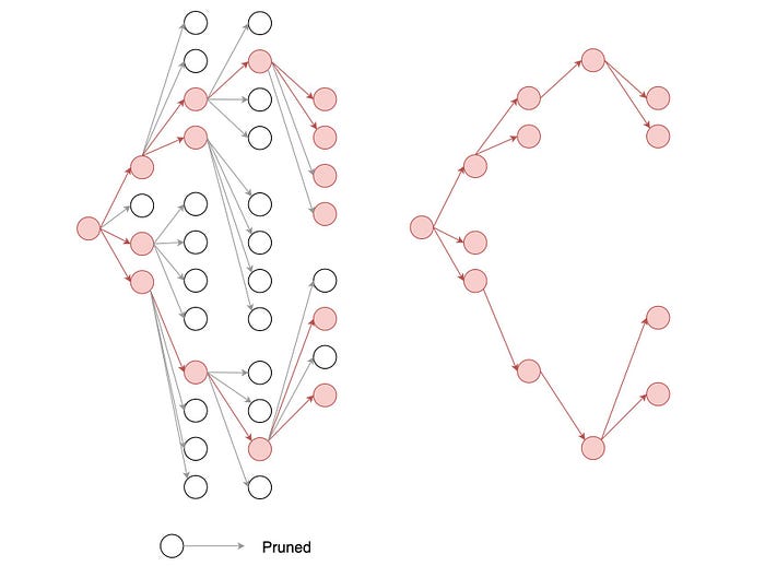
Nevertheless, the CTC implementation remains complex, in particular, handling edge cases. Fortunately, there are Baidu open-source implementation and the TensorFlow implementation on CTC loss and CTC beam-search that we can use.

Deep Speech

Next, let’s look at building a deep network specifically from what has been learned. Below is a deep network called Deep Speech.

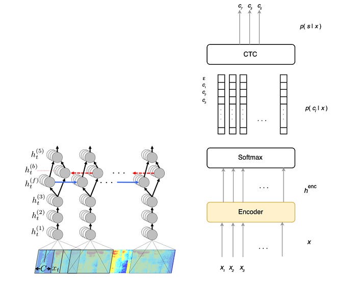
At each time step, the design above applies a sliding window to extract the power at different frequencies.

At each time step, Deep Speech applies three FC layers to extract features. Then, it is feed into a bi-directional RNN to explore the context of the speech. Deep Speech adds the results from the forward and backward direction together for each time step. Then, it applies another FC layer to transform the result. Finally, the probability for each character at each time step is computed with a softmax.

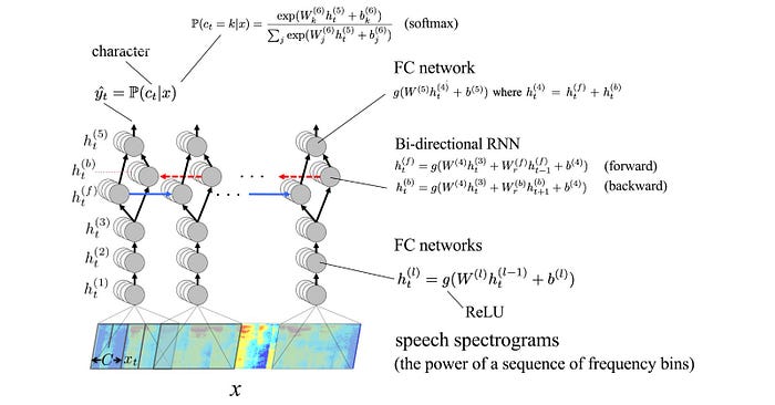
Here are the characters that are included for the probability distribution:

Then, it applies CTC and beam-search to find the most likely word sequence for the utterances.

Deep speech uses the objective function below to find the optimal sequence of characters. This objective function is based on the distribution output of the deep network, an N-gram language model and the word count of the decoded sentence. Both α and β are hyperparameters to be tunned. The language model allows us to produce grammatically sound sentences. But the deep network may be biased to create un-necessary more or fewer words than it should be. So we add a word count objective to tune the selection process.

Here is the Mozilla implementation and its Github and Baidu research on Deep Speech.

RNN Transducer

CTC predicts the distribution of characters for each audio frame.

To find the optimal word sequence, we can incorporate a language model in the beam-search as shown before. But we will not cover the detail here. (The principle will be similar to the integration of the lexicon model and the language model discussed before.) Instead, we will focus on another approach in integrating the language model concept directly into the deep network.

Basically, a language model predicts what is next based on the previous decoded words. We can expand the concept further to create a deep network that makes predictions in the context of what it has already predicted.

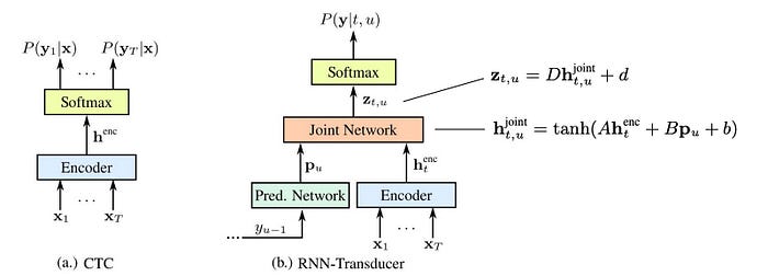
The change requires two more components: the prediction network and the joint network. The prediction network receives the previous label prediction as input and computes an output vector pu. pu depends on the last prediction which also depends on the one before. Therefore, pu actually depends on the whole sequence of previous predictions. pu can be viewed as a guess on the coming prediction based on the previous predictions. On the other side, we have an encoder that creates a dense representation of the current input. We joint both information together using the equations above. Intuitively, we form a new deep network that makes predictions based on previous contexts and the current observations. That is the same principle behind the language model. In fact, Deep Speech follows a similar principle. But Deep Speech looks at both the forward and the backward direction. This is the concept of RNN transducer which integrates a language model concept into the deep network.

Attention

Before discussing the last topic, we need to understand attention first. The picture below contains about 1M pixels. But most of our attention will likely focus on the blue-dress girl below.

When creating a context for our next prediction, we should not put equal weight on the information we collect so far. This is a big waste of computing resources. We should create a context of what we are interested in. But this focus can shift in time. For example, if we mention the word ferry, we may focus on the ticket booth behind the second street lamp instead. So how can we conceptualize this into equations and deep networks?

Before, in the RNN, we make predictions based on the new input x and the historical output context h.

For an attention-based system, we can look into the whole input x again for each step but it will be replaced with the attention.

We can visualize that the attention masks out input information that is not important for the current process.

For each input feature xᵢ, we train an FC layer with tanh output to score how important the feature i (or the pixel) is for the current time step under the previous output context. For instance, our last output maybe the word “ferry”.

Then, we normalize the score using a softmax function.

The attention Z will be the weighted output of the input features. In our example, the attention may fall around the ticket sign. The key point is we introduce an extra step to mask out information that we care less at the current step.

Listen, Attend and Spell (Encoder-Decoder)

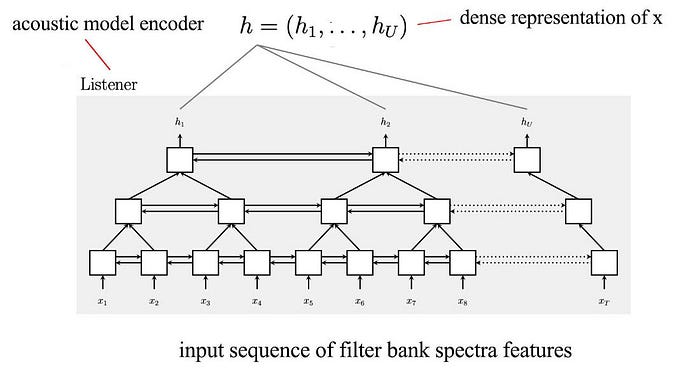
Listen, Attend and Spell (LAS) is an encoder-decoder system. It composes of an encoder (the listener at the bottom) and a decoder (the speller on the top). The encoder takes audio frames and encodes them into a denser representation. The decoder decodes it into the distributions of characters in each decoding step.

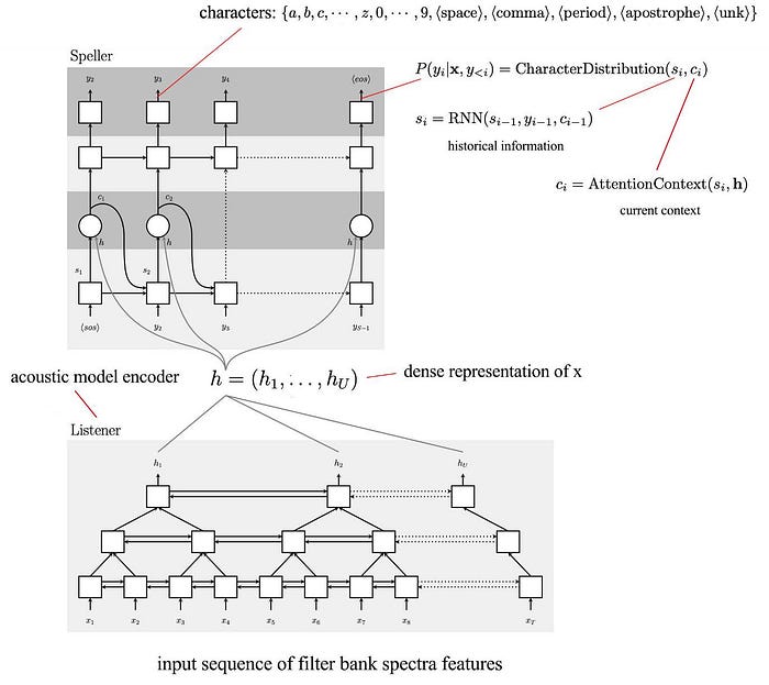
The encoder composes of pyramid layers of bidirectional LSTM. The output of the LSTM in each layer is feed into the upper LSTM layer with the time resolution reduced by a factor of two. This allows us to form a dense representation for hundreds or thousands of audio frames. It allows helps us to explore the context gradually and hierarchically.

The speller is a decoder with attention. It is implemented with LSTM transducers.

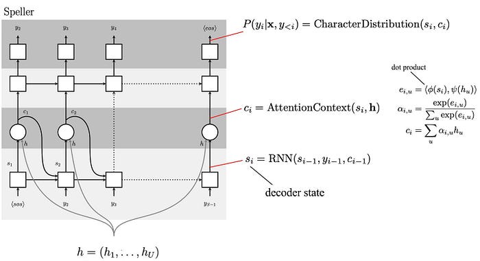
In the first step, we compute the decoder state as:

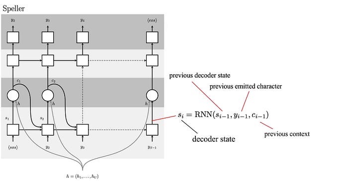
The decoder state will depend on previous decoder state, previous emitted character (the character that the speller predicted) and the previous context (discussed later) computed in the last time step.

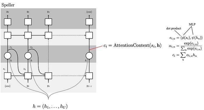
Next, we compute scores (attention) using the decoder state and the encoder state h. First, we use two MLP (Multilayer perceptron) to process the current decoder state s and h (the dense representation of the input x) further. Then we find their similarity using a dot product. This is the attention score for different components in h. We compute the softmax and use that to create the current context c. This context is a weighted output of the encoder state h based on the attention score. In short, we find what components in h should we focus on.

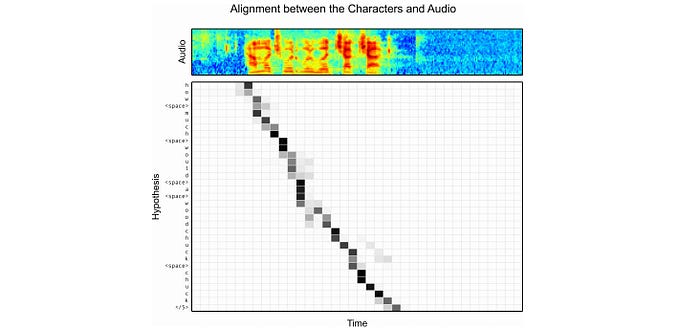
Below is the heat map correlated the attention context and the utterance. As shown, for each character output, the attention focuses on a small number of audio frames only.

Finally, the character distribution is computed with the decoder state and the attention context using MLP.

In training, LAS creates a model that maximizes the probability of the ground truth. However, during inference, the ground truth is missing and the model can suffer if the previous emitted state we use to compute the decoder state turns to be a bad prediction. Therefore, during training, instead of feeding the ground truth for next step prediction all the time, LAS sometimes samples from the previous character distribution and use that as the emitted state in the next step prediction instead. So the model is trained with the following objective instead.

In decoding, we want to find the most likely character sequence:

LAS applies a beam-search from left to right. The search maintains a set of partial possibilities. The beam is expanded with the next possible characters and then later pruned to constrain the size of the search space. A word dictionary can be used to penalize non-word spelling. But it turns out that LAS with the context concept is already good at spelling and therefore not necessary. When the <eos> token is reached, we will remove the path from the beam and added to one of the possible candidates for the later final selection. Once all the candidates are generated, we perform the last round of rescoring.

The amount of text corpus is much larger than transcripted utterance. So for the rescoring, we can put back the language model for final selection. In addition, LAS tends to create sentences with more characters than it needed, we will penalize our objective for the number of characters in the decoded text (|y|). Therefore, the objective below will be used to select the final candidate.