Speech Recognition — Weighted Finite-State Transducers (WFST)

17 min readSep 24, 2019

Previously, we developed all the necessary Lego blocks in modeling our ASR problem. They include the HMM models for the triphones, the pronunciation lexicons for words and the language models for the grammar. If the HMM models are simple and the vocabulary size is small, we can concatenate and compose them together and decode the Markov chain exactly with the Viterbi decoding.

However, for LVCSR (Large vocabulary continuous speech recognition), the models are too complex to be solved easily. We are still facing a steep hill to climb! We need to rethink how we represent all these building blocks systematically and to process them efficiently.

Overview

In this article, we apply a hierarchical pipeline concept that composes Weighted Finite-State Transducers (WFST) together. It composes multiple transducers to a single transducer and uses that to search (decode) for a grammatically-sound sentence.

Weighted Finite-State Transducers WFST is good at modeling HMM and solving state machine problems. In the ASR context, it provides a natural representation for HMM phonetic models, context-dependent phones, pronunciation lexicons, and grammars. For example, the pronunciation lexicon transducer L below decodes phone sequences into words.

Weights can be associated with edges as costs or probabilities. For example, the diagram below represents a word-level grammar transducer G in modeling a bigram language model. It calculates the likelihood of a word sequence.

The key strength of WFST is composing transducers together to build structures. Transducers encode a mapping between the input and the output label sequences. From the bottom of the diagram below, we use an HMM transducer H to recognize HMM states into context-dependent phones. By composing other transducers, namely the context-dependency, the pronunciation lexicon, and the grammar transducer, we map phones into a grammatically-sound sequence of words.

This componentize strategy makes implementation much easier with far fewer mistakes, and it can be optimized to streamline the decoding. In this article, we will develop the basic concepts first before we dig deeper into WFST. Again, the concept may first look simple or obvious but it builds up a powerful framework for ASR decoding later.

Finite State Automaton (Finite State Machine)

A finite-state automaton is a model defining a state machine with transitions between states in response to some input. The following diagram has 4 states. In the state S₁, if an input c is received, it will transit to the state S₂.

Here are the terms we need throughout this article. Note that we also call labels as symbols in this article. In ASR, we also call labels as strings.

Semirings

Let’s consider a system composed of boolean values (either 0 or 1) with operators “and” and “or”. We write the “and” operator as ・ and the “or” operator as +. Naturally, we called them the multiplication and addition operator. For any value in this system, (a + b) + c = a + (b + c) and (a・b) ・c = a・(b ・c). In fact, it fulfills all the requirement below.

This sounds obvious! But they do serve important purposes. Semiring allows a broad class of operations and algorithms applied to automata (the finite state machine). In a nutshell, Semiring enables us to develop solutions applicable to a wide range of problems.

A real number set with the + and × operators forms a Semiring also. Here are some other examples that can be used to compute probabilities and minimum path.

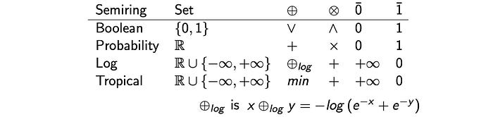
where each Semiring will define its own multiplication operator ⊗ and addition operator ⊕.

Given a state machine like the one below, the weight of a path is computed by the ⊗ operator, and the cost of an input sequence is calculated by summing up all matched paths with the ⊕ operator. For example, the cost for the input “ab” equals 1 ⊗ 1 ⊗ 1 ⊕ 3 ⊗ 3 ⊗ 1.

Here is an example of finding the sum of all path for the sequence ab in the Real semiring. Real semiring uses + operation for the ⊕ operator and × for the ⊗ operator.

By substituting different definitions for the ⊗ and ⊕, Semiring can serve different purposes. The weights in Probability Semiring are the probabilities to transit from one state to another. ⊗ (with operator ×) computes the combined probability along a path. ⊕ (with operator +) sums up the total probability of all possible paths for an input. In Log Semiring, the weights are the costs computed as the negative logs of the probabilities. ⊕ takes the negative log of its parameters as:

Tropical Semiring uses the same negative logs but with minimum function as the ⊕ operation. Computing the sum of paths in Tropical Semiring locate the minimum path.

The general solution for the sum of paths will be:

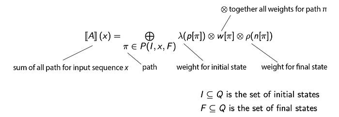
This Semiring scheme allows us to represent automata in many problem domains. For the Probability Semiring (sometimes, we also call it Real Semiring), the sum of the path is the probability of recognizing the input or the input/output sequence. For the Tropical semiring, it gives us the mechanism to find the minimum path or the most likely sequence using the Viterbi decoding.

Finite-State Acceptor (FSA)

Finite-State Acceptor is a finite representation of a possibly infinite set of labels. It matches a sequence of labels to paths between the initial and the final state. If such a path is found, this sequence of label is accepted. Otherwise, it is rejected. For example, the input sequence “abca” will be accepted while “bcb” will be rejected below.

We can add weight to each arc. This is called a weighted finite-state acceptor.

We can also add weight to the final state. For example, the final state 1 below has a weight of 2.

Empty label

ε (or “-” or <eps>) implies an empty label. Let’s demonstrate it with an example. A final state can have outbound arcs and an initial state can act as a final state. With the combination of looping and empty label, the FSA below accepts “a”, “aa”, “aaa”, … etc.

Weighted Finite-State Transducers (WFST)

A finite-state transducer (FST) has arcs labeling the input and output labels. A path through the transducer maps an input label sequence to an output label sequence. WFST is the weighted version of the finite-state transducer. If an arc has empty input or output, it will be marked with <eps>, ε or “-”.

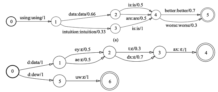
The first WFST above is a language model. Both the input and output labels are the same. Its main purpose calculates the probability for a word sequence (the grammar). For the second WFST, it is a pronunciation lexicon. It maps phones \d\ \ey\ \t\ \ax\ to “data” or phones /d/ /uw/ to “dew”. Once an input sequence is accepted, the first arc output “data” with the rest output empty labels.

The sum of all path for WFSA and WFST are respectively:

Operations

Operations can be applied to WFST regardless of what exactly it is representing or the type of Semiring. Let’s go through some popular operators quickly in manipulating WFST.

Sum (Union)

In this example, we “sum” over three FST to form a new one.

For example, we can “sum” over all the pronunciation lexicons for words to represent the lexicon covering all words in the vocabulary. In the diagram above, we also include the equation on how the sum of the path is calculated using the corresponding transducers.

Product (Concatenation)

Product concatenates FST. By concatenating WFST for words, we form a sentence.

Closure (Kleene closure)

Closure loops back WST to form a looping structure. This creates a word sequence from individual words to model a continuous speech.

Reversal

Reversal reverses the flow.

Inversion

Inversion inverts the input labels with the output labels. Instead of mapping x to y, we may y to x.

Projection

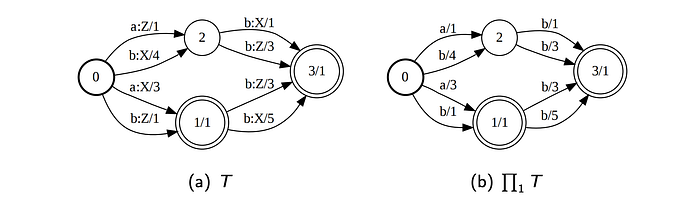
Composition

The most important operator is composition. This is the one that builds the hierarchical pipeline structure. It integrates different models into a single model.

Here we compose two WFST together:

In composition, we cycle through the arc combinations. If the output symbol of the first WFST matches the input symbol of the second WFST, we create a new arc. Here is a very simple example of composing words to a grammatically-sound sentence.

Here is another example of composing two WFST together.

Composing transducers with empty labels ε will require special attention.

Without going into details, it requires steps to ensure the final graph includes unique and valid paths.

Nevertheless, the composed WFST can be large with a lot of redundancy.

Determinization

To improve search efficiency, we can impose the WFST to be deterministic. Determinization eliminates multiple paths and each input sequence now has a unique path. It reduces the time and space in decoding an input sequence significantly. But not all WFST can be determinized.

To enforce this constraint, the transducer has to

No two arcs have the same input label from the same state (node), and
No empty input label (but some toolkit implementations like OpenFst allow this).

Determinization reduces branching when word starts where most uncertainty happens.

Minimization

Minimization turns a deterministic WFA into one with the minimal number of states. Again it simplifies the model.

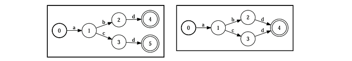
Here is another example in sharing a prefix.

We have skipped many details and insights on how composition, determinization, and minimization are done. It is a large topic. please refer to this paper if more information is needed.

More information (optional)

The composition and optimization method have many fine implementation footnotes that we purposely miss to focus on the core ideas. The good news is there are libraries to handle composition. So researchers can focus on the models rather on the composition implementations. But for those that want more details, please check out the papers and slides in the reference section. For this section here, we will mention some issues at a high level only. We intend to create awareness rather than explaining them in details.

Composition with Epsilon

Epsilons make the composition more difficult. For example, for the composed transducer below, it can be and should be simplified to the blue path only. We need to filter out all the redundant and unnecessary path.

This can be achieved by introducing a Filter F between the composition.

Epsilon-Removal

Epsilon-Removal removes ε-transitions from the input transducer and produces the equivalent epsilon-free transducer. This helps WFST efficiency but not all can be done and some may cause more harms.

Weight-pushing

Weights can either be can be pushed towards the initial or final states.

In another example below, the weight on a path is normalized. The total outbound weight of a node equals to 1. Any path score remains the same before the push.

Weights can be redistributed to the head with pushing. This makes the pruning algorithm works better since the weight can be look-ahead early. This is helpful in a lexicon or language model.

Token Passing

Backtracing the optimal path can be tedious. We can build a word tree representing the word sequence from the starting state. Backtrace pointer points to last best word sequence or if a word boundary is detected, it points to the current word sequence.

WFST with ASR

To decode an audio clip into the most likely sequence of words, we use WFST to represent the HMM phones model (bottom diagram below), the pronunciation lexicon (the middle) and the grammar (the top) respectively.

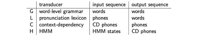
The following is the four transducers with the corresponding types of input and output. We use these transduces to decode streams of HMM states into a grammatically-sound word sequence.

Here is a conceptual example of decoding context-dependent phones to a sequence of words. First, we decode CD phones into CI phones (3 states/phone usually). Then we convert it to word sequence.

But we don’t do it in separate steps. We compose and optimize transducers together to form a single WFST to map HMM states to a sequence of words. All the compositions and optimization are pre-compiled. Therefore, major load is offloaded during decoding. These are the beauties of WFST.

In addition, new transducers can be added to enhance or to extend the current pipeline. As long as it is a WFST, we can compose them together. This gives an abstract but powerful mechanism in extending the capability of ASR. We can apply different WFST operations like sum, product, inversion, and composition to create a large WFST.

H ◦ C ◦ L ◦ G composition

The ASR decoder use the composition of H ◦ C ◦ L ◦ G to form a single transducer as the speech recognizer where

G is the grammar/language model acceptor.
L is the pronunciation lexicons.
C is the context-dependent relabeling (convert context-dependent phone to context-independent phone).
H is the HMM structure (outputting context-dependent phones — HMM internal state sequence).

Grammar Transducer G

The following is an oversimplified bigram language model transducer G.

The diagram below is a trigram model with the vocabulary {u, v, w} using backoff. Let’s say we start from the previous words u v. If the input is w, we will take arc ③ if p(w|u, v) > 0. The probability of this transition will be modeled by the trigram which equals p(w|u, v). The output word sequence will be “uvw” (including the previous words uv”).

But as mentioned in the previous article, the data in the trigram model can be sparse. Even p(w|u, v) equals zero in the training data, this probability can be non-zero in the real world. To handle this, we will apply backoff from the trigram model to a bigram model in estimating p(w|u, v), i.e. p(w|u, v) = α(u, v) p(w|v). To accept “w” as the next word, we will take the path ① ②. In arc ①, we take the backoff and fall back to a bigram model. The transition probability will be α(u, v) in a typical backoff model. Then we take path ② with probability p(w|v) according to the bigram model. So the combined probability equals α(u, v) p(w|v). Since arc ① takes an empty input, the word sequence after taking arc ② is “uvw” (including the previous words uv”).

Lexicon Transducer L

This is the lexicon for the word “data” that takes care of different pronunciations of the word.

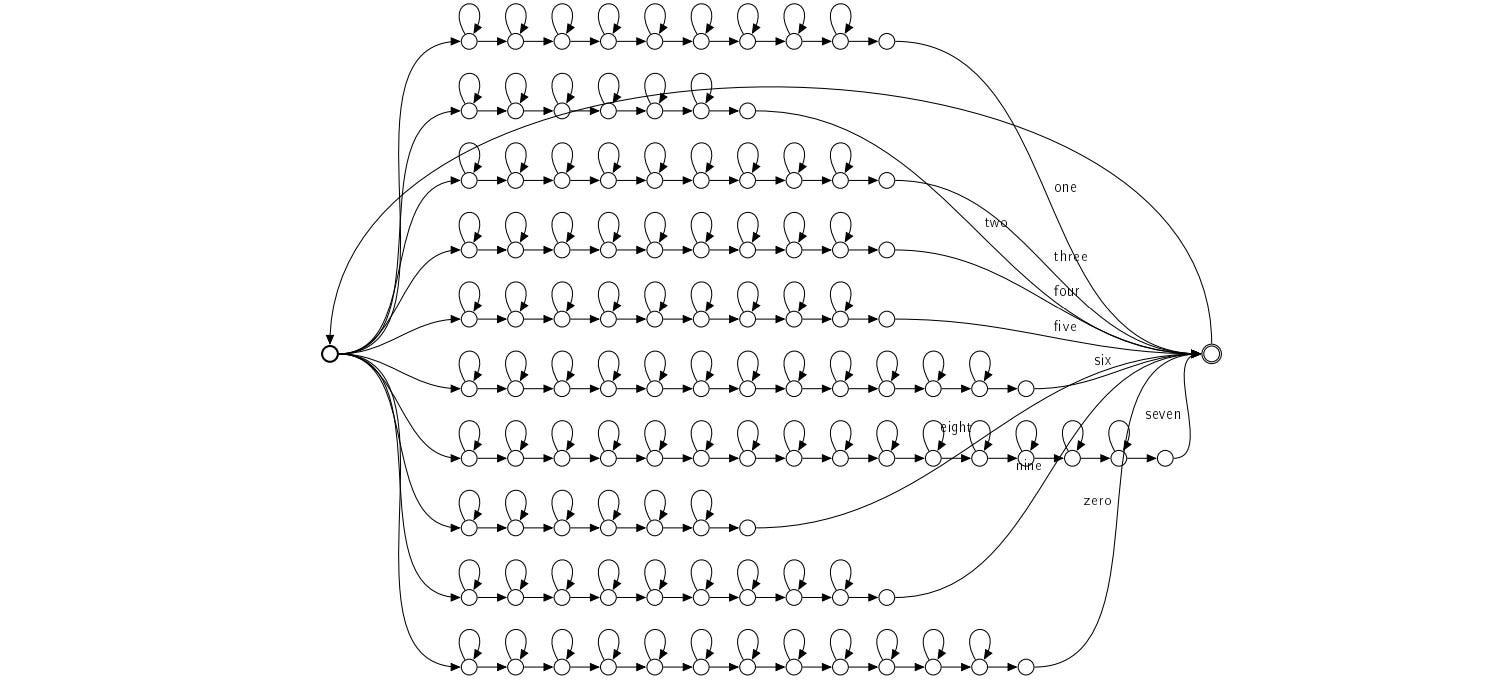
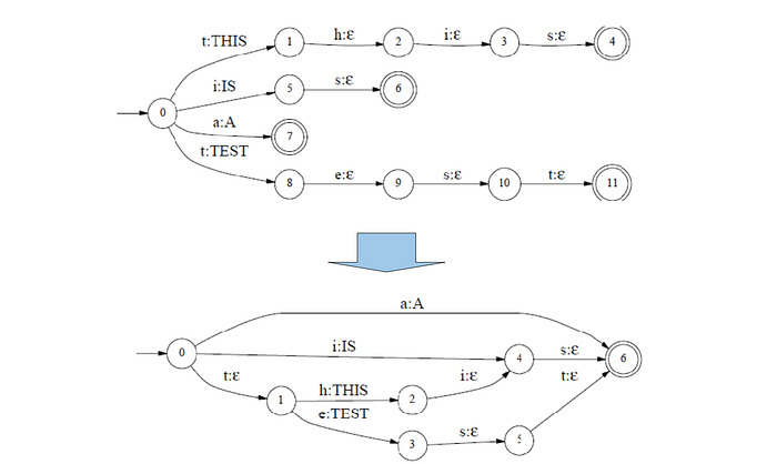
Here is the lexicon that union 7 words in the vocabulary.

A sequence of phones may map to different words. To differentiate different scenarios, we add additional disambiguation symbols at the end when ambiguity happens.

Here is a more complex example. The phone ax #1 will terminate the word “A” and will not continue to identify the word “ABOARD”.

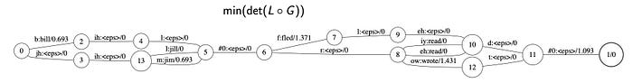
L ◦ G composition

Here is a simple example in composing L and G with optimization applied.

Context-dependent Transducer

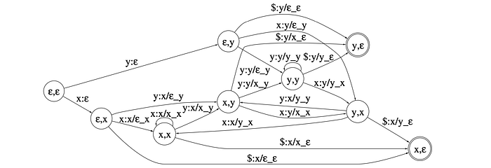
The first FSA below is context-independent (CI). The second diagram is the transducer in mapping context-independent labels (like phoneme) to context-dependent (CD) labels. For example, in the arc between state 2 and 3, the label is x:x/y_x. x/y_ x indicates x is preceded by y followed by x. So we are converting x into the CD label “x/y_ x”.

(Note: e means empty string here).

But the transducer C in H ◦ C ◦ L ◦ G takes CD labels and output CI labels. So C is actually the inverse of the WFST above. Again this is a more complex example.

HMM transducer

The HMM transducer maps HMM states into CD triphones. As a demonstration, the following composed WFST maps HMM states to phonemes. The number on the input label is the ID for the HMM states.

Composed recognizer

We compose H, C, L, and G together to form a single decoding/search graph. The following is how we optimize it through determinization and minimization.

There are other fine details including the handling of empty labels and disambiguation symbols. Please refer to Mohri’s paper for details.

Decoder

Let’s come to the final part on decoding an utterance. Consider we have an utterance composed of N audio frames. We can model the triphone transition of the utterance

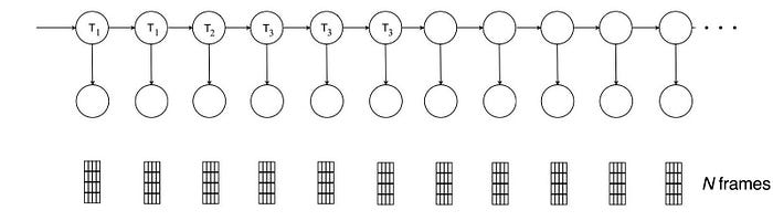
with a Finite-State Acceptor (FSA) U. The diagram below shows the FSA for an utterance composed of 3 audio frames with 4 HMM states.

The first label in each transition (arc) corresponds to an HMM triphone state for time t. The second value is the corresponding negated and scaled acoustic log-likelihoods. That is, according to the acoustic GMM model associated with a triphone, we score its likelihood at time t. U and our composed transducers form a new search space.

However, we don’t compose them together. The graph will be too big to store or to perform a full search. Transducer composition is simply an optimization step. We can always apply Viterbi decoding to transducers to find the most likely path. The catch is if we want to scale the solution, we need to perform beam-pruning on the Viterbi algorithm. Pruning is a key part of the decoding. To make it even more effective, perform determinization and weight pushing. It allows language model look-ahead for a better pruning.

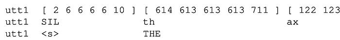
However, we can use other searching or decoding algorithms including A* search (a depth-first search compared to the Viterbi algorithm which is a breath-first search) in searching the decoding space. To scale, we just need to apply approximation, like the beam-pruning in limiting the size of the search. Below is an example on the detected triphone states, the phoneme, the alignment and the word decoded.

Word Lattice Generating

Instead of finding the best path in the search graph, say using the beam-pruned Viterbi decoding, we can search for the space to generate an N-best list. The search result can be represented as a Word Lattice, like the one below.

Or, we can generate the search result as an FSA. This graph can be conceptualized as an extremely aggressive pruning of the search space.

Then, we apply a second recognizer to find the best word sequence. With a smaller number of candidates to consider or to model, the second recognizer can be far more complex and take longer time per choice. For instance, the second recognizer usually utilizes a longer-span language mode instead of a bigram or a trigram model. (More information on generating a lattice graph solution is found here.)

Applications

Now, let’s look at the models of the transducers. (This example is from Mohri’s paper.)

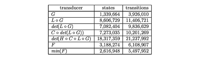
First-Pass Transducers

This application is building an integrated, optimized speech recognition transducer for a 40K-word vocabulary in the North American Business News (NAB) task. The models used are: