What do we learn from single shot object detectors (SSD, YOLOv3), FPN & Focal loss (RetinaNet)?
In part 2, we will have a comprehensive review of single shot object detectors including SSD and YOLO (YOLOv2 and YOLOv3). We will also look into FPN to see how a pyramid of multi-scale feature maps will improve accuracy, in particular for small objects that usually perform badly for single shot detectors. Then we will look into Focal loss and RetinaNet on how it solve class imbalance problem during training.
Part 1: What do we learn from region based object detectors (Faster R-CNN, R-FCN, FPN)?
Part 2: What do we learn from single shot object detectors (SSD, YOLO), FPN & Focal loss?
Part 3: Design choices, lessons learned and trends for object detections?
Single Shot detectors
Faster R-CNN has a dedicated region proposal network followed by a classifier.

Region-based detectors are accurate but not without a cost. Faster R-CNN processes about 7 FPS (frame per second) for PASCAL VOC 2007 testing set. Like R-FCN, researchers are streamlining the process by reducing the amount of work for each ROI.
feature_maps = process(image)
ROIs = region_proposal(feature_maps)
for ROI in ROIs
    patch = roi_align(feature_maps, ROI)
    results = detector2(patch)    # Reduce the amount of work here!
As an alternative, do we need a separate region proposal step? Can we derive both boundary boxes and classes directly from feature maps in one step?
feature_maps = process(image)
results = detector3(feature_maps) # No more separate step for ROIs
Let’s look at the sliding-window detector again. We can slide windows over feature maps to detect objects. For different object types, we use different window shapes. The fatal mistake of the previous sliding-windows is that we use the windows as the final boundary boxes. For that, we need too many shapes to cover most objects. A more effective solution is to treat the window as an initial guess. Then we have a detector to predict the class and the boundary box from the current sliding window simultaneously.

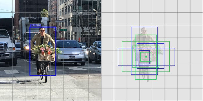
This concept is very similar to the anchors in Faster R-CNN. However, single shot detectors predict both the boundary box and the class at the same time. Let’s do a quick recap. For example, we have an 8 × 8 feature map and we make k predictions at each location. i.e. 8 × 8 × k predictions.

At each location, we have k anchors (anchors are just fixed initial boundary box guesses), one anchor for one specific prediction. We select the anchors carefully and every location uses the same anchor shapes.
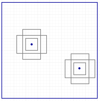
Here are 4 anchors (green) and 4 corresponding predictions (blue) each related to one specific anchor.
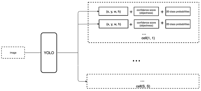
In Faster R-CNN, we use one convolution filter to make a 5-parameter prediction: 4 parameters on the predicted box relative to an anchor and 1 objectness confidence score. So the 3× 3× D × 5 convolution filter transforms the feature maps from 8 × 8 × D to 8 × 8 × 5.
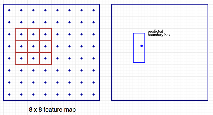
In a single shot detector, the convolution filter also predicts C class probabilities for classification (one per class). So we apply a 3× 3× D × 25 convolution filter to transform the feature maps from 8 × 8 × D to 8 × 8 × 25 for C=20.
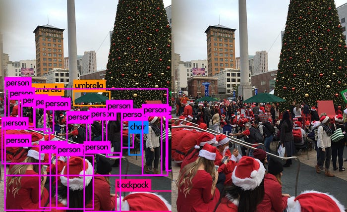
Single shot detector often trades accuracy with real-time processing speed. They also tend to have issues in detecting objects that are too close or too small. For the picture below, there are 9 Santas in the lower left corner but one of the single shot detectors detects 5 only.
SSD
SSD is a single shot detector using a VGG16 network as a feature extractor (equivalent to the CNN in Faster R-CNN). Then we add custom convolution layers (blue) afterward and use convolution filters (green) to make predictions.

However, convolution layers reduce spatial dimension and resolution. So the model above can detect large objects only. To fix that, we make independent object detections from multiple feature maps.

Here is the diagram showing the dimensions of feature maps.
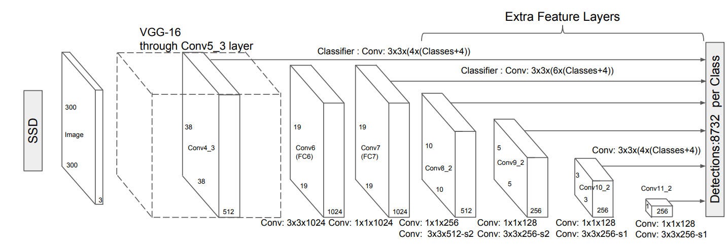
SSD uses layers already deep down into the convolutional network to detect objects. If we redraw the diagram closer to scale, we should realize the spatial resolution has dropped significantly and may already miss the opportunity in locating small objects that are too hard to detect in low resolution. If such problem exists, we need to increase the resolution of the input image.

YOLO
YOLO is another single shot detector.
YOLO uses DarkNet to make feature detection followed by convolutional layers.

However, it does not make independent detections using multi-scale feature maps. Instead, it partially flattens features maps and concatenates it with another lower resolution maps. For example, YOLO reshapes a 28 × 28 × 512 layer to 14 × 14 × 2048. Then it concatenates with the 14 × 14 ×1024 feature maps. Afterward, YOLO applies convolution filters on the new 14 × 14 × 3072 layer to make predictions.
YOLO (v2) makes many implementation improvements to push the mAP from 63.4 for the first release to 78.6. YOLO9000 can detect 9000 different categories of objects.

Here are the mAP and FPS comparison for different detectors reported by the YOLO paper. YOLOv2 can take different input image resolutions. Lower resolution input images achieve higher FPS but lower mAP.

YOLOv3
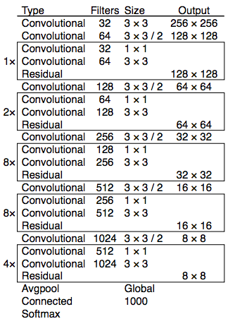
YOLOv3 change to a more complex backbone for feature extraction. Darknet-53 mainly compose of 3 × 3 and 1× 1 filters with skip connections like the residual network in ResNet. Darknet-53 has less BFLOP (billion floating point operations) than ResNet-152, but achieves the same classification accuracy at 2x faster.
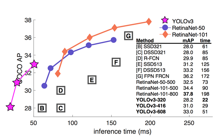
YOLOv3 also adds Feature Pyramid (discussed next) to detect small objects better. Here is the accuracy and speed tradeoff for different detectors.
Feature Pyramid Networks (FPN)
Detecting objects in different scales is challenging in particular for small objects. Feature Pyramid Network (FPN) is a feature extractor designed with feature pyramid concept to improve accuracy and speed. It replaces the feature extractor of detectors like Faster R-CNN and generates higher quality feature map pyramid.
Data Flow
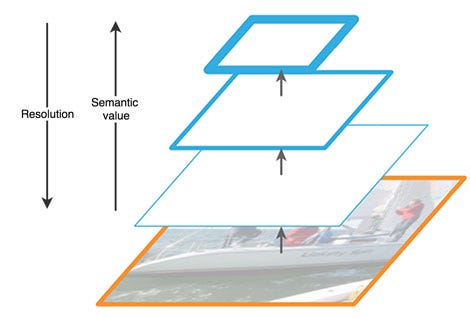
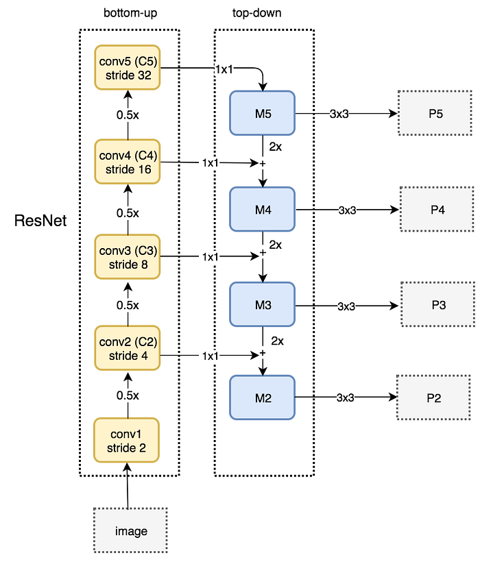
FPN composes of a bottom-up and a top-down pathway. The bottom-up pathway is the usual convolutional network for feature extraction. As we go up, the spatial resolution decreases. With more high-level structures detected, the semantic value for each layer increases.
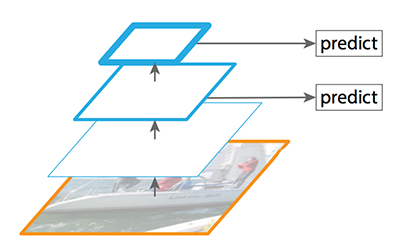
SSD makes detection from multiple feature maps. However, the bottom layers are not selected for object detection. They are in high resolution but the semantic value is not high enough to justify its use as the speed slow-down is significant. So SSD only uses upper layers for detection and therefore performs much worse for small objects.
FPN provides a top-down pathway to construct higher resolution layers from a semantic rich layer.
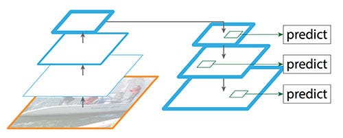
While the reconstructed layers are semantic strong but the locations of objects are not precise after all the downsampling and upsampling. We add lateral connections between reconstructed layers and the corresponding feature maps to help the detector to predict the location betters.
The following is a detail diagram on the bottom-up and the top-down pathway. P2, P3, P4 and P5 are the pyramid of feature maps for object detection.
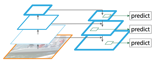
FPN with RPN
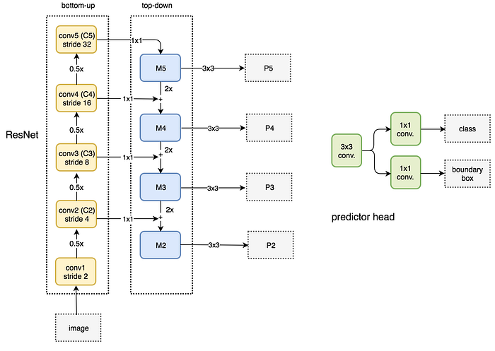
FPN is not an object detector by itself. It is a feature detector that works with object detectors. The following feed each feature maps (P2 to P5) independently to make object detection.
FPN with Fast R-CNN or Faster R-CNN
In FPN, we generate a pyramid of feature maps. We apply the RPN (described above) to generate ROIs. Based on the size of the ROI, we select the feature map layer in the most proper scale to extract the feature patches.

Hard example mining
For most detectors like SSD and YOLO, we make far more predictions than the number of objects presence. So there are much more negative matches than positive matches. This creates a class imbalance which hurts training. We are training the model to learn background space rather than detecting objects. However, we need negative sampling so it can learn what constitutes a bad prediction. So, for example in SSD, we sort training examples by their calculated confidence loss. We pick the top ones and makes sure the ratio between the picked negatives and positives is at most 3:1. This leads to a faster and more stable training.
Non-maximal suppression in inference
Detectors can make duplicate detections for the same object. To fix this, we apply non-maximal suppression to remove duplications with lower confidence. We sort the predictions by the confidence scores and go down the list one by one. If any previous prediction has the same class and IoU greater than 0.5 with the current prediction, we remove it from the list.
Focal loss (RetinaNet)
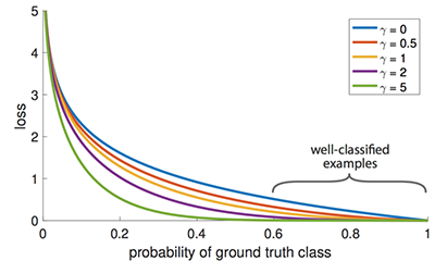
Class imbalance hurts performance. SSD resamples the ratio of the object class and background class during training so it will not be overwhelmed by image background. Focal loss (FL) adopts another approach to reduce loss for well-trained class. So whenever the model is good at detecting background, it will reduce its loss and reemphasize the training on the object class. We start with the cross-entropy loss CE and we add a weight to de-emphasize the CE for high confidence class.
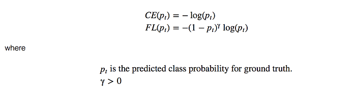
For example, for γ = 0.5, the focal loss for well-classified examples will be pushed toward 0.
Here is the RetinaNet building on FPN and ResNet using the Focal loss.

