RL — Reinforcement Learning Terms
Reinforcement learning observes the environment and takes actions to maximize the rewards. It deals with exploration, exploitation, trial-and-error search, delayed rewards, system dynamics and defining objectives.
Agent
The system (like robots) that interacts and acts on the environment.
Controller
Same as an agent.
Policy
A policy defines how an agent acts from a specific state. For a deterministic policy, it is the action taken at a specific state.

For a stochastic policy, it is the probability of taking an action a given the state s.

Rewards
Reward r(s, a) defines the reward collected by taking the action a at state s. Our objective is to maximize the total rewards of a policy. A reward can be the added score in a game, successfully turning a doorknob or winning a game.
Notation and example

Episode
Playing out the whole sequence of state and action until reaching the terminate state or reaching a predefined length of actions.
Value function (state-value function)
The value function of a state V(s) is the total amount of expected rewards that an agent can collect from that state to the end of the episode.
Action-value function
The action-value function Q(s, a) is the total amount of expected rewards of taking an action from the state until the end of the episode.
Model (system dynamics)
A model describes how an environment may change upon an action from a state p(s’ | a, s). This is the system dynamics, the law of Physics, or the rule of the game. For a mechanical problem, it is the model dynamics on how things move.
Discount rate γ
Discount rate values the future rewards at the present value. It γ is smaller than one, we value future rewards less at the current value.

Model-Free RL
In model-free RL, the system dynamics is unknown or not needed to solve the task.
Model-based RL
We use the known model or the learned model to plan the optimal controls in maximizing rewards. Or we can collect those sampled controls to train a policy and hope that it may be generalized to other tasks that we have not trained before.
Monte Carlo Method
Monte Carlo methods play through a completed episode. It computes the average of the sample returns from multiple episodes to estimate value functions. Or it uses the following running average to update the result.

Monte Carlo control
We use the Monte Carlo method to evaluate the Q-value function of the current policy and find the optimal option by locating the action with the maximum Q-value functions.

Actor-critic
Actor-critic combines the concept of Policy Gradient and Value-learning in solving an RL task. We optimize the actor which based on Policy Gradient to determine what actions to take based on observation. However, Policy Gradient often has a high variance of gradient that hurts convergence. We introduce a critic in evaluating a trajectory. This critic makes use of past sampled experience and other techniques that reduce variance. This allows the actor to be trained with better convergence.
Policy Gradients
We refine our policy for making actions more likely when we expect it to have large expected rewards (or vice versa).
Natural Policy Gradients
It is similar to Policy Gradients. But Natural Policy Gradient uses a second-order optimization concept which is more accurate but more complex than the Policy Gradient which uses the first-order optimizer.
Sample efficiency
Sample efficiency relates to how many data samples needed in optimizing or finding the solution. Tasks requiring physical simulation can be expensive and therefore it is an important evaluation factor in selecting RL algorithms.
On-policy learning v.s. off-policy learning
In on-policy learning, the target policy is the same as the behavior policy, i.e. the behavior policy used to sample actions to observe the rewards is the same as the target policy to be optimized. Mathematically, the behavior policy is the sampling distribution in the expectation function below. As shown, we sample from θ to compute the expectation. This is the gradient we use to optimize the target policy θ (L.H.S.) using gradient ascent.

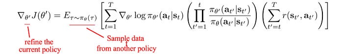
Off-policy learning has separate policies for behavior policy and target policy. Many on-policy methods have corresponding off-policy methods using importance sampling (details in 1, 2). In the example below, we are using a slightly staled policy θ’ as the behavior policy. We recalibrated its observed rewards with importance sampling to compute the rewards under the target policy θ. And θ’ will regularly synchronize with θ to improve the accuracy for the recalibrated rewards.
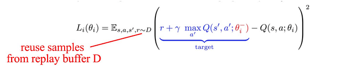
DQN is also off-policy. As shown, samples are drawn from a replay buffer.
These examples improve sampling efficiency by reusing old sampled data. But other designs can be applied to address different issues. For example, we can design a better behavior policy to make a better exploration strategy other than ε-greedy or we can design different policies to improve model convergence.
Markov Decision Process (MDP)

It composes of states, actions, the model P, rewards and the discount factor. Our objective is to find a policy that maximizing the expected rewards.
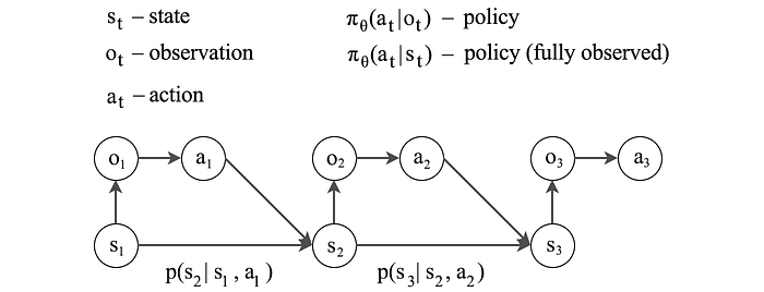
Partially Observable Markov Decision Process POMDP
Not all states are observable. If we have enough states information, we can solve the MDP using the states we have (π(s)). Otherwise, we have to derive our policy based on those observables (π(o)).
Prediction
Predict the future states when taking certain actions.
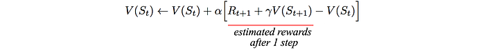
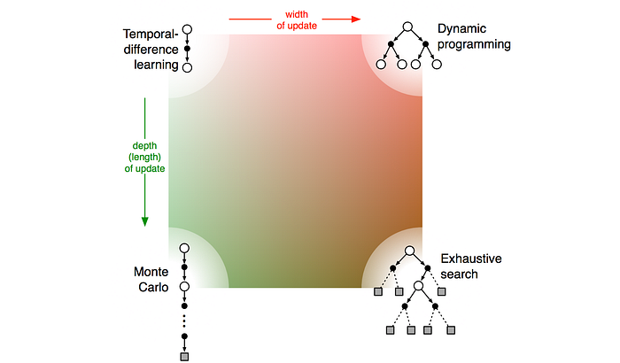
Temporal-Difference Learning (TD)
Instead of completing the whole episode like the Monte Carlo:
We rollout k-steps and collect the rewards. We estimate the value function based on the collected rewards and the value function after k-steps. Below is a 1-step TD learning. We find our the reward after taking one action. The equation below is a running average for V using TD.
Monte-Carlo samples the state-action space vertically in the depth direction. Dynamic programming acts more in the width direction. TD will have the shortest depth and width.
Planning
We use the system dynamics (model) to generate simulated experience and use them to refit the value functions or the policy.
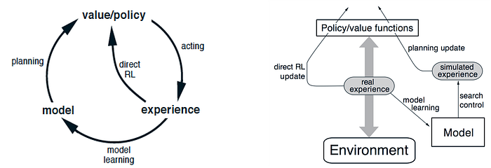
The difference between learning and planning is one from real experience generated by the environment and one from simulated experience by a model.
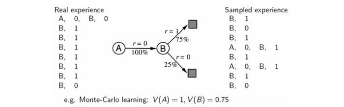
On the left side below, we collect real experience using the Monte-Carlo method. V(A) = 0 from the real experience. However, from the real experience, we can build a model on how states are transited. Using this model, we can create sampled experience on the right. For example, with this sampled data, V(A) = 1 which is better than the one calculated from the real experience.
Linear system with additive Gaussian noise
The next state is a Gaussian distribution with the mean computed from a linear dynamic model.

Q-learning
We learn the Q-value function by first taking an action (under a policy like epsilon-greedy) and observe the rewards R. Then we determine the next action with the best Q-value function.

The Q-value function is learned as:

Linear Gaussian controller
A Linear Gaussian controller samples action from a Gaussian distribution with the mean computed from a linear model.

Linear Gaussian dynamics
The next state is modeled from a Gaussian Distribution using a linear model.

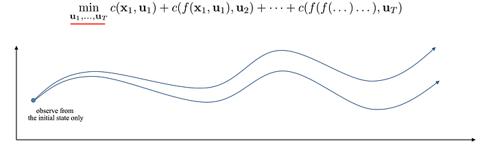
Trajectory optimization
Finding the best state and the action sequence that minimizing a cost function.
Open-loop system
We observe the initial state of a system and plan actions to minimize a cost function.
Close-loop system
We observe the initial state of a system and plan the actions. But during the course, we can observe the next state and readjust any actions. For a stochastic model, this allows us to readjust the response based on what actually occurred. Hence, a close-loop system can be optimized better than an open-loop system.
Shooting methods
Optimize trajectory based on an open-loop system. Observe the initial (first) state & optimize the corresponding actions.
For a stochastic system, this is suboptimal because we do not readjust the actions based on the observed states where we transit to.
Collocation methods
Optimize trajectory based on a closed-loop system which we take actions based on the observed states. We manipulate both actions and states in optimizing the cost function.

Imitation learning
Imitate what an expert may act. The expert can be a human or a program which produce quality samples for the model to learn and to generalize.
Inverse reinforcement learning
Try to model a reward function (for example, using a deep network) from expert demonstrations. So we can backpropagate rewards to improve policy.
Math terms
Taylor series

In vector form:

where g is the Jacobian matrix and H is the Hessian matrix.
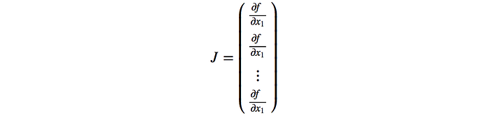
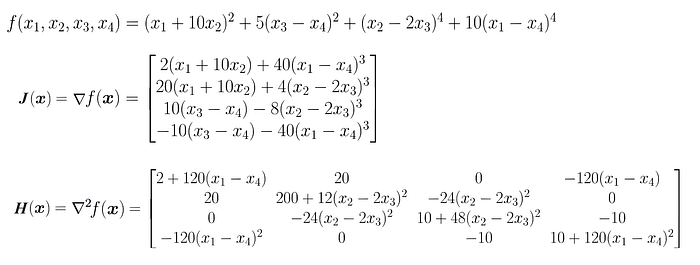
Jacobian matrix
Hessian matrix

Examples:
KL-divergence
In deep learning, we want a model predicting data distribution Q resembling the distribution P from the data. Such a difference between two probability distributions can be measured by KL Divergence which is defined as:

Positive-definite matrix
Matrix A is positive-definite if

for all real non-zero vector z.
Questions
Why do we use stochastic policy in Policy Gradients?
Stochastic policy models the real world better as we act on incomplete information. In addition, a small change of action can have a big swing on the rewards. The expected rewards will have a much steeper curvature with a deterministic policy. This destabilizes models easily and makes it vulnerable to noise. A stochastic policy will have a smoother surface with less sharp cliff since it tries out combinations of actions which smooth out the total rewards. So stochastic policy will work better with optimization methods like gradient descent.
